| [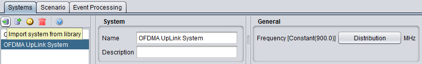](https://wiki.cept.org/uploads/images/gallery/2026-04/wguxUeEfzyjU48f9-image.png) | [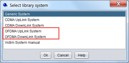](https://wiki.cept.org/uploads/images/gallery/2026-04/9F0y94LlRPrMPa5p-image.png) |
| (a) | (b) |