9 OFDMA module

• 9.1 Introduction
• 9.2 OFDMA system tab
• Introduction
• 9.4 Positioning
• 9.5 Link-to-system level mapping
• 9.6 Achieved bit rate
• 9.7 DL C/I calculation
• 9.8 UL C/I calculation
• 9.9 UL calculation of the UE frequencies
• 9.10 OFDMA UL power control
• 9.11 Pathloss Correlation

9.1 Introduction

The current OFDMA module has been designed for a Long Term Evolution (LTE) network from 3GPP ‎[12]. Therefore E-UTRA RF coexistence studies can be performed with Monte-Carlo simulation methodology.

The general simulation assumptions are presented in this section to provide a guideline on how to perform coexistence simulations. The OFDMA DL (downlink) LTE algorithm implemented in SEAMCAT assumes a 100% loaded system and each user is allocated with a fixed number of resource blocks. This is equivalent to modelling a Round Robin scheduler with full buffer traffic model and a frequency reuse of 1/1 (i.e. Single Frequency Network is assumed). The OFDMA algorithm as implemented in SEAMCAT takes into account the intra system interference into the reference cell, caused by UEs located in adjacent cells and using the same RBs but also caused by UEs located in the reference cell which are using different RBs. The OFDMA UL (uplink) LTE algorithm implemented in SEAMCAT is similar to the OFDMA DL LTE algorithm with one exception. In the OFDMA, UL system it is possible to  load the system with a set number of resource blocks rather than only 100% load like in the OFDMA DL system (see 9.3.6).

The network layout is similar to the one used for CDMA. The methodology assumes that the UEs are deployed randomly in the whole network region according to a uniform geographical distribution. The wrap around technique is employed to remove the network deployment edge effects.

Note that if the OFDMA is a DL interferer, the OFDMA is simulated as in “traditional” simulation with the BSs transmitting at full power. This decreases the simulation time of a full OFDMA simulation. In OFDMA DL interferer case, only the position of the BSs will be calculated because full transmit power is assumed. For all other simulations (including UL) scenarios full OFDMA network simulation is required. Consequently, some of the input parameter of the GUI interface have been grey-out when the OFDMA DL interferer case is selected.

Since it is arguable that some simulation assuming a rural environment would not need to assume full power transmission (i.e. full loaded network) when the system is DL and interferer, you may need to manipulate either the input power or the spectrum mask (or both) in order to simulate the DL interferer case for rural deployment.

9.2 OFDMA system tab

Introduction

Whether you want to simulate OFDMA UL or OFDMA DL, you can import

 from the system library (Figure 199 – (a)), the cellular system you want (Figure 199 – (b)). You can also export

 the characteristics of your OFDMA network to the library for later reuse. 

(a)	(b)

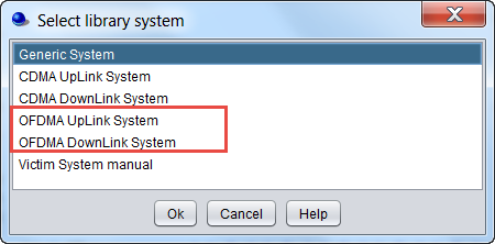
Figure 199: Selection of a OFDMA cellular network from the system library

9.4 Positioning

See section ‎7.5, common to CDMA and OFDMA on the positioning of BSs and MSs.

9.5 Link-to-system level mapping

A look up table is used to map throughput in terms of spectral efficiency (bps per Hz) with respect to calculated SINR (= C/(I+N)) (dB) level. This link level data (bitrate mapping) is user selectable and can be modified depending on the simulation to perform.

 

9.6 Achieved bit rate

The achieved bit rate is calculated as follows:

 (Eq. 45)

The achieved aggregate bit rate is calculated over all the mobiles connected to the reference cell.

9.7 DL C/I calculation

The relationship between the contributors of the interference in a OFDMA network is illustrated in Figure 205.

 

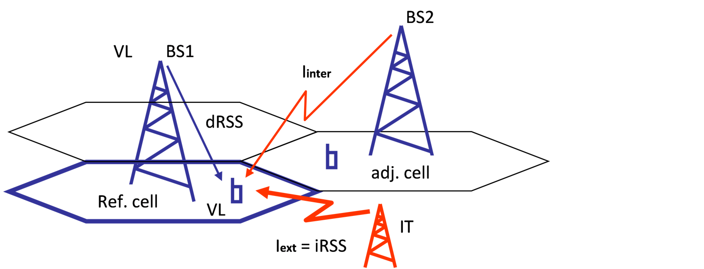
Figure 205 illustrates the interference mechanism in the OFDMA module where the inter-system or also called self interference is noted “Iinter” and the interference from an “external” interference system is referred to as “Iext”. In the SEAMCAT OFDMA implementation, the term “BS” and “cell” have the same meaning.

 

The C/I calculation in DL is calculated as                                                                             

    (Eq. 46)

where C(j,k) is the received power at the k-th user from the serving BS, i.e., the j-th BS

                                                            (Eq. 47)

and where  is the power of resource block and effective_pathloss is defined as in Section ‎7.6.1.

I(j,k) is the sum of the interference power

                                                                                         

 (Eq. 48)

where

 

• I_inter (j,k) is the adjacent cell interference (i.e. from the same victim system, i.e. denoted inter-system interference;

• I_ext(j,k) is the interference from external interfering system(s) in adjacent channel, i.e interference power into this resource block including ACIR;

• N is the noise floor.

 

 (Eq. 49)

 (Eq. 50)

I_ext(j,k) is the interference to the the victim UE_j,k from N interfering link transmitters (ILT). Note that the ACIR (Adjacent Channel Interference Ratio) is implicitly taken into account when both unwanted and blocking mechanism are summed in the computation. The unwanted and blocking are defined as follow

 

 

       (Eq. 51)

 

for each of the victim UE_j,k’s frequency where the DL information is received. The ILT can be any generic systems or a BS/UEs of a cellular system.

  (Eq. 52)

 

at the victim system frequency. Where N_RB is the number of RBs (i.e. subcarriers) requested per UE, and M is the maximum number of RBs per BS.

  (Eq. 53)

where NoiseFigure_UE is the noise figure of a UE.

9.8 UL C/I calculation

The C/I calculation in UL is calculated so that C(j,k) is the received power from the UE_j,k at the j-th BS.

                                   (Eq. 54)

where P_t is the transmit power of the UE in dBm (see UL Power control below) and effective_pathloss is defined as in Section ‎7.6.1..

The total interference to a UL cellular system is derived from

 (Eq. 55)

where

• I_inter is the interference coming from UEs of the same system but from adjacent cells, i.e. the inter-system interference from other cells. Since a fully orthogonal system is assumed, only UEs  which transmit in the same frequency subcarriers will introduce interference to each other, hence only UEs in other cells with the same k index are considered;

• I_ext(j,k) is the interference from external interfering system(s) in adjacent channel;

• N is the noise floor.

                                         

 (Eq. 56)

               

 (Eq. 57)

 

I_ext(j,k) is the interference to the the victim BS_j from N interfering link transmitters (ILT), where

 

 (Eq. 58)

for each of the victim BS_j’s frequency where the UL information is received. The ILT can be any generic systems or a BS/UEs of a cellular system.

         

  (Eq. 59)

 

at the victim system frequency. Where N_RB is the number of RBs (i.e. subcarriers) requested per UE, and M is the maximum number of RBs per BS.

 

(Eq. 60)

 

where NoiseFigure_BS is the noise figure of a BS.

9.9 UL calculation of the UE frequencies

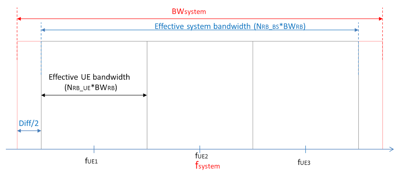
The frequency of the UE in UL is calculated as follow

(Eq. 61)

with Diff taking into account for any difference between the BWsystem and the effective bandwidth ( ) so that

(Eq. 62)

where

• F_UE: Centre frequency of the UE;

• F_system: Frequency of the system (i.e. the network);

• _BW system : Bandwidth of the system;

• N_RB_UE: Number of Resource Blocks (RB) per mobile;

• N_RB_BS: Number of RB for the BS;

• BW_RB: Bandwidth of the RB;

• N_UE: Number of UEs in the system (calculated as NRB_BS/NRB_UE);

• Index_link: Index of the specific link UE to serving BS (input to SEAMCAT). Index = [0, NUE-1].

9.10 OFDMA UL power control

In OFDMA UL, the power control is applied to the active users (i.e. the mobile users with specific RBs) so that the UE Tx power is adjusted with respect to the effective path loss (i.e. based on the MCL) to the BS it is connected to. In 3GPP ‎[12], the UL power control is defined so that the UE transmit power is set such as: 

 

 (Eq. 63)

where:

• Pt is the UE Tx power in dBm;

• P_max is the maximum transmit power in dBm;

• R_min is the minimum power reduction ratio to prevent UEs with good channels to transmit at very low power level. R_min is set by P_min / P_max.

• CL is the effective path loss in dB for the UE from its serving BS;

• CL_x-ile is the x-percentile effective path loss (plus shadowing) value. CL_x-ile is defined here as the value in the CDF, which is greater than the effective path loss of x percent of the MSs in the cell from the BS (i.e. it corresponds to the parameter “power Scale Threshold”. It is set by default to 0.9, but you can change it;

• γ is assumed to equal to 1 by default in SEAMCAT.

 

With this power control scheme, the 1-x percent of UEs that have a path-loss greater than CL_x-ile will transmit at P_max, i.e. are not power controlled. Annex ‎A15.6 provides further information about the implementation and the usage of the OFDMA UL power control.

9.11 Pathloss Correlation

The concept of a simple correlation model for shadow fading has been widely adopted in LTE co-existence studies mostly employed in uplink case. The propagation attenuation is modelled as the product of the path loss and the shadow fading. The shadow fading is well approximated by a log-normal distribution. Let z denotes shadow fading in dB with zero mean and variance σ². Then the shadow fading of path from one UE to the i-th BS is expressed as

   (Eq. 64)

 

where a²+b²=1 and x and y_i are independent Gaussian distributed variables, both with zero mean and variance σ² . y_i and y_j for are independent as well.

Figure 207 presents how to set-up the pathloss correlation in SEAMCAT (only available for OFDMA). The panel is similar for the OFDMA DL and UL.

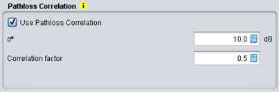
Figure 207: Illustration of the pathloss correlation – input parameters

 

 

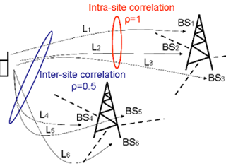
Thus, the correlation coefficient of the shadow fading from one UE to two different BSs, i.e., the i-th and j-th BS, is

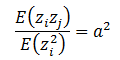(Eq. 65)

 

 In most LTE studies,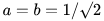  is assumed ‎[10]. For cellurar systems with three-sector antennas, the shadowing correlation between sites (equivalent to BS in Omni antenna system) is of 0.5 and correlation between sectors of the same site is consequently of 1.