# 8.6 CDMA Downlink - simulation algorithm
# 8.6.1 Simulation Methodology
The main goal of the downlink power control in SEAMCAT is to calculate the total BS output power and the success rate (% of calls with no link quality degradation) for a given snapshot of the system. BS output power is a key parameter in the scenarios where CDMA is the interferer. Success rate, on the other hand, is crucial in CDMA victim scenarios. One possible way to analyze the impact of other system interference on CDMA is to compare the success rates in the presence and absence of external interference.
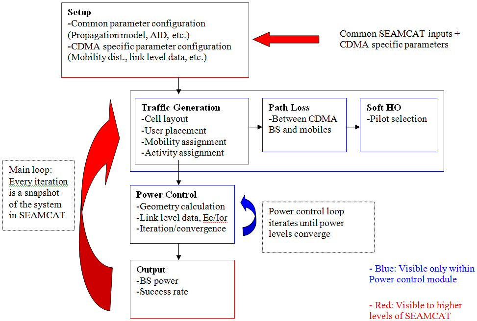
A snapshot of the mutually existing systems is modeled at each event generation in SEAMCAT. Hence, at each event generation the power control algorithm should also be run for the CDMA cell, whether it is the victim or the interferer. This is illustrated in Figure 194. The setup block is inherited from the higher layers of SEAMCAT and consists of initializing the system parameters. The next step involves the generation of traffic for power control, calculation of appropriate path losses within the CDMA cell layout and determination of soft handover states. Power control is then performed by utilizing the link level data via an iterative process. Finally, necessary outputs are generated and fed into the interference calculation modules in SEAMCAT.
[](https://wiki.cept.org/uploads/images/gallery/2026-04/YP7nS30VpVbHEcRd-image.png)
**Figure 194: DL Power Control Simulation Methodology – Overview**
For simplicity, the CDMA downlink power control methodology is described for omni-cells. However, extension to multi-sector cells is straightforward. In a multi-sector configuration, each sector should be treated in the same way a cell is treated in the omni configuration.
# 8.6.2 Traffic Generation
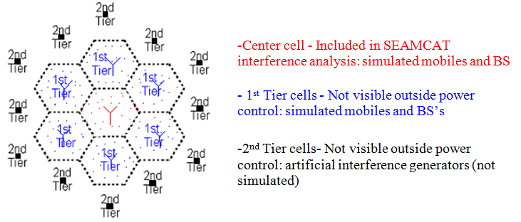
While the BS output power and the outage ratio is likely to be calculated for a single CDMA cell, accurate modelling of power control requires the consideration of inner-system interference generated by the surrounding tiers of CDMA cells. The significance of other cell interference in CDMA requires that at least two tiers surrounding the cell of interest be considered. However, BS power and outage statistics will only be collected from the center cell, which has the most accurate interference background (two surrounding tiers). Cells surrounding the center cell will not be visible to the higher levels of SEAMCAT and will only be used to generate the inner-system other-cell interference background for the center cell (Figure 195).
[](https://wiki.cept.org/uploads/images/gallery/2026-04/AVpV5tB0J1kqIROC-image.png)
**Figure 195: Cell layout for power control**

The power control simulation time increases with the number of cells for which power control algorithm is run. One way to reduce the simulation time is to simulate only the center cell and the first tier around it with actual power control algorithms and use artificial interference generators for the second tier as shown in Figure 195. More specifically, the BS’s in the center cell and the first tier go through the power control algorithms and calculate the precise power they need to transmit. Whereas, the BS’s in the second tier are assigned an output power level to generate interference into the center cell and the first tier. If the output power level set for the second tier is reasonable, this approach will speed up the simulation considerably without sacrificing much from accuracy. Possible methods to determine the appropriate artificial interference level will be addressed later in the paper. Nevertheless, if more accurate results are desired, the second tier can also be simulated using actual power control. In that case, a third tier with artificial interference generators would further increase accuracy by presenting the second tier with a more realistic interference background. However, given the considerations on complexity, the layout shown in Figure 195 presents the most appropriate balance between simulation speed and accuracy.
Since higher levels in SEAMCAT consider only a single CDMA cell, the cell layout shown in Figure 195 may need to be generated separately in the power control module. It is expected that the UE placement be done consistently with SEAMCAT’s existing algorithms. However, once the UEs are placed, their mobility assignment should also be done. Actual mobility of the UEs cannot be simulated easily in a static simulation, but the effects of mobility on the channel power can be modeled in a limited sense. While the UEs will be treated at fixed locations within each snapshot, each will be assigned a speed to determine their channel conditions (fast fading), which will be used in the determination of their channel power requirements. This allows the flexibility to simulate various system configurations (fixed, highway, pedestrian, etc.).
# 8.6.3 Soft Handover
A user may simultaneously be connected to multiple BS’s in CDMA based systems (soft handover). Since soft handover affects the amount of power transmitted by each BS to a certain user, it is necessary to determine whether the UE is served by a single BS or multiple BS’s. The actual determination of the soft handover state of a user and the corresponding channel power requirements may get complicated. Hence, a simplified soft handover algorithm is presented next, which captures the essence of soft handover effects while avoiding implementation of complex algorithms.
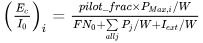
Base stations that are connected to a user are included in the “active set” of that user. A base station is initially selected to be in the “active set” based on the strength of its pilot signal versus the interference background. Each base station broadcasts a certain fixed percentage of its maximum power on the pilot channel. The interference background consists of the non-orthogonal energy received on the other channels of the base stations within the active set and the total broadcast power of the base stations that are not in the active set. The BS selection criterion, “pilot Ec/Io” is then defined as
[](https://wiki.cept.org/uploads/images/gallery/2026-04/0aom4TPKs0y7JtbV-image.png) *(Eq. 34)*
with the following definitions:
- *Ec* is the chip energy received from ith BS;
- *Io* is the spectral density of total received interference;
- *pilot\_frac* is the fraction of BS power allocated to pilot;
- *P*max,*I* is the maximum receivable power from ith BS (max BS transmit power\*path loss);
- *W* is the system bandwidth;
- *Pj* is the total received power from jth BS;
- *F* is the mobile station noise figure;
- *N0* is the thermal noise power density;
- *Iext* is the external interference (out of system).
Based on this selection criterion, the following simplified soft handover algorithm can be employed to assign soft handover states to each user:
For each user:
1. Add the BS with the strongest corresponding Ec/Io to the active set;
2. Add the BS with the second strongest corresponding Ec/Io to the active set if its Ec/Io is within 4 dB of the strongest Ec/Io.
Then the soft handover state of a user becomes the number of BS’s in its active set, which is either one or two. Note that in actual systems, the active set of a user may have more than 2 BS’s. However, in order to develop a unified methodology that can simulate various implementations of CDMA based systems and to avoid overwhelming complexity, this simplified approach is suggested. Several standards (including UMTS) present similar methodologies for simulations.
# 8.6.4 Power Control
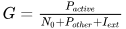
As far as SEAMCAT is concerned, the actual CDMA power control algorithm looks merely like a black box that maps link quality to channel power. However, the mapping is not simply one-to-one. Depending on the conditions of the mobile user, the same link quality can map to different channel power requirements. A key parameter that determines the condition of a user is called the “geometry”. The higher the geometry, the more favorable the UE’s condition is. The geometry is defined as:
[](https://wiki.cept.org/uploads/images/gallery/2026-04/cIY8CPNbQy7cqIan-image.png) *(Eq. 35)*
with the following definitions:
- Pactive is the total power received from BS’s in the active set;
- *No* is the thermal noise;
- *P*other is the total power received from BS’s not in the active set;
- *I*ext is the external Interference (out of system).
The fractional power levels found in the link level data are defined for each user (channel) as:
[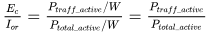](https://wiki.cept.org/uploads/images/gallery/2026-04/Wi23GOne9Y4buPz1-image.png) *(Eq. 36)*
with the following definitions:
- *Ptraff\_active* is the total received traffic channel power from BS’s in the active set
- *Ptotal\_active* is the total power received from BS’s in the active set
Ptotal\_active is the sum of the total received power from the BS’s in the active set including their pilot, overhead and all traffic channels. Whereas Ptraff\_active includes only the traffic channel power that is received from the BS’s in the active for the particular user. In other words, a user’s Ec/Ior shows the fraction of the total received power that is used for voice communication with that user. Based on this definition, the amount of traffic channel power received from a BS for a particular user can be derived from the Ec/Ior requirements reported in the link level data.
If user has only 1 BS in the active set (simplex), the power received from the BS is:
[](https://wiki.cept.org/uploads/images/gallery/2026-04/XywpaHBJvG43gYH6-image.png) *(Eq. 37)*
If user has 2 BS’s in the active set (2-way soft handover), power received from one of the BS’s is then:
[](https://wiki.cept.org/uploads/images/gallery/2026-04/duZVAGYMskbXPONw-image.png) *(Eq. 38)*
Note that symmetry between the two soft handover legs (links with BS’s in the active set) is assumed. Therefore, when a user is connected to two BS’s, it receives equal power from each link. The determination of the traffic channel power levels for each user cannot be done in a single step. The inherent assumption in equations 37 and 38 is that Ptotal\_active is known. However, Ptotal\_active itself is the sum of the pilot, overhead and all traffic channel power levels received from the BS’s in the active set. Therefore, an iterative process is required to determine the individual traffic channel received power levels.
[](https://wiki.cept.org/uploads/images/gallery/2026-04/mspuin7Xdpys7IdM-image.png)
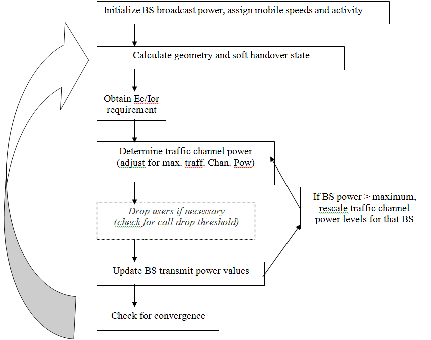
**Figure 196: Power Control Loop**
Figure 196 shows how the power control loop operates. The initial step is to initialize each BS in the cell layout (figure 1) by assigning total broadcast power levels. A figure around 70% of maximum BS power is appropriate. Note that for the simulated BS’s, the total BS power will be updated at each iteration by the power control loop. After enough iterations, the power levels will converge to the correct values.
Once the initialization is complete, geometry and soft handover state for each user can be calculated based on the initial values of the BS broadcast levels. Then the Ec/Ior requirement for each active user can be obtained from the link level data using its mobile speed assignment, calculated geometry and soft handover state. Equations 37 and 38 can then be used to get the received traffic channel power levels for each user. Path loss information can then be used to determine the corresponding transmit channel power levels. However, the calculated transmit traffic channel power levels should be checked against the maximum allowable traffic channel power and transmit/receive levels should be adjusted if necessary. As a result of such an adjustment, a user may not meet its Ec/Ior requirement. Based on a “call drop threshold”, such a user may be removed from the system if it meets the following criterion:
[](https://wiki.cept.org/uploads/images/gallery/2026-04/0hgGMg3DpvxUj7YB-image.png) *(Eq. 39)*
The call drop threshold is set such that dropping a call is limited to extreme circumstances (thresholds less than 2dB are not recommended) and kept mostly as a safety measure to avoid a single user hogging the BS resources. In an actual system, calls are not dropped at the instant they fail to meet their link quality target. The system will tolerate quality degradation up to certain durations and at the same time avoid a single user to sacrifice the overall system performance by consuming all the BS resources (max. traff. chan. pow. setting). In fact, for systems that employ sufficient control of maximum traffic channel power, call drops may be avoided completely within the power control loop. Eventually, users not meeting their Ec/Ior target will be evaluated when the success rate of the system is calculated.
Once the transmit traffic channel levels are calculated, the broadcast power of each BS should accordingly be updated. If the total broadcast power of a BS turns out to be greater than its maximum allowable level, all traffic channels served by that BS should be scaled down so that the maximum BS power constraint is met. The scaling factor that should be applied to the traffic channel power levels can easily be calculated as:
[](https://wiki.cept.org/uploads/images/gallery/2026-04/bZbyoKC5yBoxQOF8-image.png) (Eq. 40)
where:
- *Pmax* is the maximum allowable BS power
- *Pcalculated* is the actual calculated BS broadcast power (including pilot and overhead).
Scaling is only done if Pcalculated > Pmax and it is done only on the traffic channels; pilot and overhead power levels remain at a constant percentage of the maximum allowable BS power. For channels that go through the scaling, achieved Ec/Ior levels may not match the required Ec/Ior levels. Therefore, call drop criterion (if used) shown in equation 6 should also be checked after the scaling. The process is outlined in Figure 199.
This process describes a single iteration of the power control loop. After all the traffic channel power levels are determined and the BS levels are updated, the process should be repeated (with the new, more accurate BS broadcast levels). Convergence of the traffic channel power levels should be checked at the end of each iteration. The loop can be terminated once the traffic channel power of every simulated user in the network converges to the desired precision.
Signaling and other errors in power control are considered in the link level simulations. System level simulations do not consider additional errors and assume that each user is served with the required power level that is determined from link level data, provided that the BS has enough power to do so and the maximum traffic channel limit is not exceeded.
# 8.6.5 Success rate
The power control loop terminates when every BS broadcast power converges and traffic channel power level for every user is calculated. Therefore, both the BS output power and the success rate for the cell of interest (center cell in Figure 198) can be calculated. BS output power is the sum of the power in pilot, overhead and all traffic channels. Success rate is the percentage of calls that do not suffer quality degradation. The following process can be used to calculate both output metrics:
i. Power control loop is terminated (traffic power converges for every user)
ii. Final BS transmit power levels are calculated (sum of all traffic, pilot and overhead)
iii. Total BS broadcast power for the cell of interest is determined
(For each active user in the cell of interest)
iv. Final geometry is calculated based on BS power levels calculated in ii.
v. Traffic Ec/Ior target is determined based on geometries calculated in iv.
vi. Achieved Ec/Ior is calculated based on BS power levels calculated in ii.
vii. Success criterion is checked
[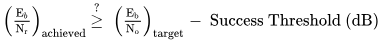](https://wiki.cept.org/uploads/images/gallery/2026-04/TYeSD4ZYQyMIZzD7-image.png) *(Eq. 41)*
viii. Success rate is determined for the cell of interest
Success Threshold is usually a small figure such as 0.5dB. Users who miss their Ec/Ior targets by more than the threshold suffer link quality degradation. Note that if call drops occurred within the power control loop, they should also be considered when success rate is determined:
[](https://wiki.cept.org/uploads/images/gallery/2026-04/zmFbK0YnsH852Flp-image.png) *(Eq. 42)*