7 Cellular network simulation

• 7.1 Introduction
• 7.2 CDMA overview
• 7.3 OFDMA overview
• 7.4 TDD vs FDD simulation
• 7.5 Cellular network positioning
• Introduction
• 7.5.1 System
• 7.5.2 System layout - reference cell selection
• 7.5.3 System layout preview
• 7.5.4 Mobile station
• 7.5.5 Base station
• 7.6 CDMA/OFDMA commonalities
• 7.6.1 Pathloss and Effective Pathloss
• 7.6.2 Measure interference from entire cluster
• 7.6.3 Wrap around feature and implementation

7.1 Introduction

Whereas traditional simulation of non-CDMA or non-OFDMA systems is carried out in SEAMCAT by taking two pairs of transmitters-receivers and estimating signals received between them separately (i.e. without any form of feed-back influence), the simulation of cellular systems requires a much more complex process of power controlling in a fully loaded system, including impact from two tiers of neighbouring cells and, for victim cellular systems, the attempt by the system to level-out the interference impact.

There are two different types of Monte-Carlo model that could be employed: a ‘static’ model, also referred to as a ‘snapshot’ model, and a ‘dynamic’ model. In a cellular network, connections will frequently arrive and leave the network during a given period of time. This causes fluctuating traffic and power levels. Principally, it is possible to carry out a dynamic Monte-Carlo taking into account this fluctuating traffic in real time. It can account for dynamical statistical characteristics; however it is extremely time consuming to run. In cases, where many scenarios need to be investigated, such long runtimes could become restrictive. Therefore, the snapshot model is preferred in such cases and selected for SEAMCAT. This model sets up a random distribution of users based on one instant in time in connection with a network configuration and considered service characteristics. A set of statistics which accurately reflects these scenarios is derived by simulating several such snapshots.

To investigate the coexistence of a mobile radio network with another radio technology in SEAMCAT, a snapshot of both victim and interfering systems is modeled at each event generation in SEAMCAT, which generates transmit power, interference levels as well as the probability of link success of the victim system for a given number of users at a time instant. It captures a snapshot of the UE powers in the network and the number of user links which can be successfully carried given these powers. In order to analyze the impact of the interfering network on the victim one, the success rates of the victim network in the presence and absence of the interfering system are compared.

The term UE or MS are used interchangeably in this manual. You should review and modify the input parameters of the cellular network for the particular scenario that is being simulated and more detailed can be found in publications such as [6], [7] or [8].

7.2 CDMA overview

When simulating CDMA systems, SEAMCAT performs power controlling in a fully loaded system of all the MSs so that the impact from the neighbourhing two tiers is included (inter-cell interference), for victim CDMA systems, and the system level-out the inter-cell and external interference impact.  The balancing of the overall system is performed by the CDMA power control algorithm.

When the CDMA system is the interferer, the UEs are balanced only once, the transmit powers and positions of relevant transmitters (BS or MS, depending on scenario) are used as interefering link transmitters for calculating the iRSS. If the CDMA system is a victim, the power balancing is done first without any external interferer, where the number of connected CDMA UEs is estimated, and then the external interferer is introduced and the CDMA system is re-balanced again. Afterwards the number of served users, compared with that before the introduction of interference was introduced, allows estimating impact of interference in terms of excess outage brought to the system. The combination of the above is applied when both victim and interferer systems are CDMA.

The term "CDMA" is used in this manual and in SEAMCAT environment in general to refer to any radio technology that employs the Code Division Multiple Access modulation scheme. The specific CDMA standard (e.g. CDMA2000-1X, or W-CDMA/UMTS) can be selected by incorporating the appropriate link level curves into the simulation scenario. Furthermore, at present, only the interference impact of/on "voice" can be studied using SEAMCAT.

7.3 OFDMA overview

The simulation of OFDMA systems is similar to that of the CDMA systems, except that after the overall two-tiers cellular system structure (incl. wrap-around) is built and populated with mobiles, OFDMA replaces the CDMA power tuning process with an iterative process of assigning a variable number of traffic sub-carriers and calculating the overall carried traffic per base station.

The OFDMA module has been designed for a Long Term Evolution (LTE) network from 3GPP TR36.942 ‎[10]. Therefore E-UTRA RF coexistence studies can be performed with Monte-Carlo simulation methodology. 

7.4 TDD vs FDD simulation

Note that TDD (Time Division Duplex)/FDD (Frequency Division Duplex) simulations are scenario dependent meaning that the direction of the interferer (UL or DL) to the victim will be studied. In this context, the time dependency is not simulated as it is not important. Therefore, SEAMCAT can already simulate this, since the worst case scenario is to be considered i.e. a FDD UL or DL scenario should give similar results as a TDD UL or DL simulation. Note however that to simulate TDD systems, the correct TDD characteristics would have to be filled in.

7.5 Cellular network positioning

Introduction

5 panels characterised the positioning of a cellular system. This panel is the same whether a CDMA (UL/DL) or OFDMA (UL/DL) is simulated.

 

7.5.1 System

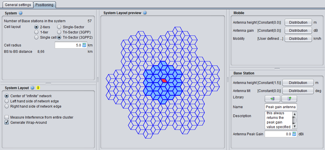
Initially macro-cellular environment was implemented in SEAMCAT, but with time more flexibility was given to the tool to reproduce various topology options in cellular network (Figure 176). Cell sites are laid out in a hexagonal grid. Sites with omni-directional antennas are placed in the middle of the cells as depicted in Figure 172 and sites with tri-sector antennas are placed at the edge of the cells, where each site covers three cells. Figure 173 shows one of these cell sites (small hexagons in dashed lines) and that the arrows demonstrate the antenna orientation of each cell. The BS to BS distance (also referred as inter-site distance in the literature) is D. The cell radius R is equal to D/sqrt(3) in the omni-antenna case and is equal to D/3  in the tri-sector antenna case. Both suburban scenario and urban scenario can be modeled with this cell configuration. The scenarios differ only in propagation conditions and in the cell radius.

A wrap around cluster is used to reduce the number of cells required in the simulations and consequently to enable faster simulation run times. The number of cell sites in the cluster is assumed to be 19 (19 cells in the case of omnia-antenna and 57 cells in the case of tri-sector antenna), which appears to be appropriate for SEAMCAT simulation (see Section ‎7.6.3 for further details on wrap-around technique). 

Figure 172: Macro-Cellular CDMA Network Deployment with Omni Antenna	Figure 173: Macro-Cellular CDMA Network Deployment with Tri-Sector Antenna

 

 

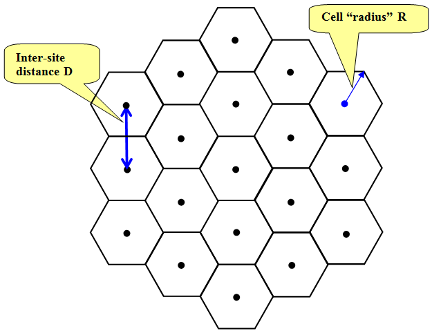
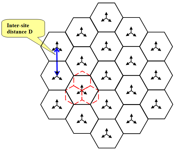
Therefore SEAMCAT supplements a single considered CDMA / OFDMA cell with its Base Station (BS) two tiers of virtual cells to form a 19 cell (57 cell for tri-sector deployment) cluster, which is then populated with a certain number of mobile stations (MS) and a power control algorithm is then applied for balancing overall system, see Figure below: 

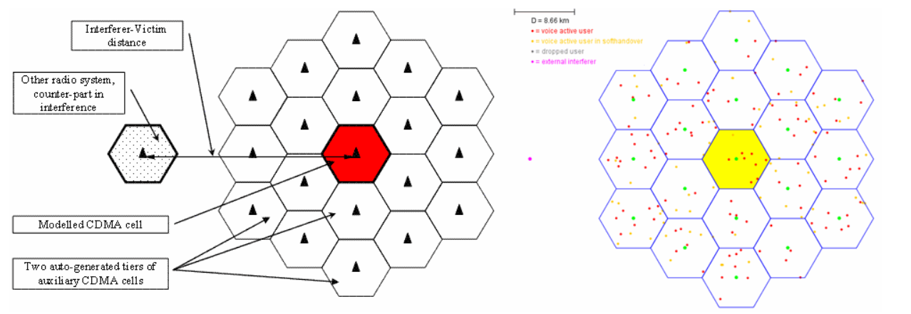
Figure 174: 19 cells omni setup

CDMA and OFDMA module shares common platform like the positioning of the cellular layout. The celular topology in SEAMCAT is composed of the “Cell layout” and the “Cell radius”a shown in Figure 176.

In the “Cell Layout” you can select 2 tiers, 1 tier or single cell layout. In addition, you can select between Omni directional (single sector),  tri-Sector (3GPP) and tri-Sector (3GPP2).

 The “Cell Radius” (km) is the size of the cell and defines also the BS to BS distance (i.e. inter-site distance). 

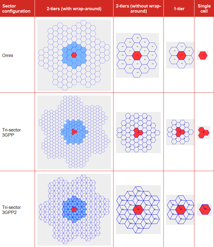
Figure 176: Overview of the topology options in cellular network

 

Two types of hexagonal grids are used to represent cellular layout, there is the 3GPP (http://www.3gpp.org/) and the 3GPP2 (http://www.3gpp2.org/). The differences are illustrated in Figure 177 (3GPP) and in Figure 178 (3GPP2). The fundamental principal of the two approaches is that they share the same commonality for the BS to BS. Based on this same value, it is possible to extract the relationship of the cell range and cell radius between the two approaches.

Within the CEPT work, it is more common to use the 3GPP hexagonal grid, ECC Repport 82 ‎[6] and ECC Repport 96 ‎[7].

Figure 177 presents an example of the 3GPP approach:

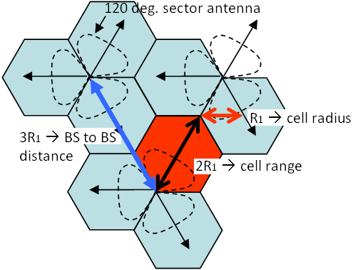
Figure 177: 3GPP illustration of the Cell Radius, Cell Range and BS to BS distance

What is important is that the BS to BS station distance be the same between the 3GPP and the 3GPP2 approach, i.e. where 3R₁ = 2h which is equivalent to R = sqrt(3) R₁. 

From there it is possible to extract the cell radius in SEAMCAT.

 

Table 21: Example of the distances relationship between 3GPP and SEAMCAT

In summary, according to Figure 179 below, the Table 22 shows the current different definitions for sector, cell and radii:

 

 

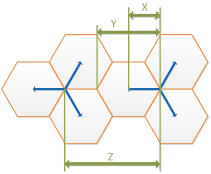
Figure 179: Different definitions for sector, cell and radii

 

 

 

7.5.2 System layout - reference cell selection

A singe cell consists of several MSs connected to their serving BS. The reference cell is a single cell that is surrounded by two tiers of virtual cells to form a 19 cells (or 57 cells for tri-sector deployment) cluster. This cells clutter is then populated with a certain number of MSs. The reference cell is by default at the center of the network, but you can modify it by selecting any cells you want. Part of configuring a CDMA or OFDMA network is selecting the reference cell. In SEAMCAT it is possible to choose between two network configurations (3GPP and 3GPP2, see Figure 176).

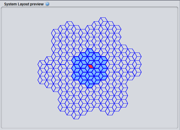
The reference cell in Figure 180 is used to calculate the effects of interference and to measure results and all non reference cells are used to provide a proper interference background to the reference cell.  You can click on the cell that should be used as reference cell when gathering results. The red cell is the current selection.

Figure 180: System layout - reference cell selection

 

 

 

 

 

 

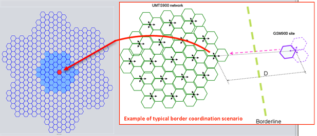
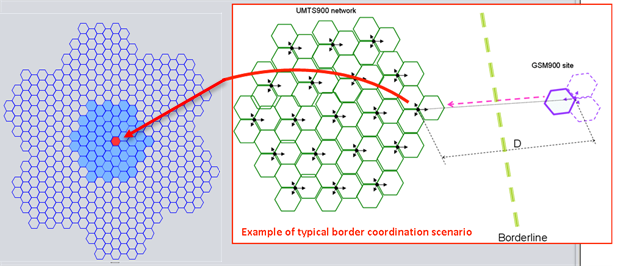
 Figure 181: Example on how to set up the system layout to reproduce a border coordination scenario

7.5.3 System layout preview

You have the possibility to see a preview of the network you are simulating. You can click on the cell that should be used as reference cell when gathering results. The red cell is the current selection. 

 

 

7.5.4 Mobile station

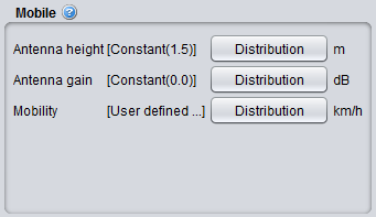
Figure 183: Cellular system – Mobile station GUI 

 

 

 

 

7.5.5 Base station

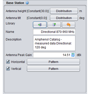
Figure 184: Cellular system – Base station GUI

 

 

 

 

 

7.6 CDMA/OFDMA commonalities

7.6.1 Pathloss and Effective Pathloss

Path loss between each user and BS needs to be calculated within the cellular layout. In SEAMCAT, there is a distinction between the raw pathloss and the effective pathloss. The effective pathloss considers the minimum coupling loss (MCL) as defined in 3GPP. The MCL is the parameter describing the minimum loss in signal between BS and UE or UE and UE in the worst case and is defined as the minimum distance loss including antenna gains measured between antenna connectors. Note that the effective path loss includes shadowing.

The effective pathloss is defined such as:

                  (Eq. 32)

where:

• G_Tx : antenna gain at the transmitter (Tx) in dBi.

• G_Rx : antenna gain at the receiver (Rx) in dBi.

The MCL is an input parameter to SEAMCAT. Typical values of MCL can be found in 3GPP documents (3). By default this value is 70 dB (i.e. typical value for Macro cell Urban Area BS <-> UE for frequency of 2000 MHz, e.g., there is a difference between 900 MHz and 2500 MHz with respect to MCL.) when defining the victim or interferer OFDMA system, but the default MCL value for generic interferer is set to 0 dB when assessing the interference between victim and interferer (ILT -> VLR path).

7.6.2 Measure interference from entire cluster

For a CDMA network used as an interferering network, when the “Measure interference from entire cluster” button is checked, all the transmitters of the CDMA network are used when simulating the interference (i.e. all 19/57 BS or all UEs in all the cells) to simulate the external interference. When it is not checked, it is only the reference cell which is the interferer. This feature only applies when a CDMA network is the source of interference.

When the interferer is OFDMA, it is assumed that the interference comes from the entire cluster and never from the reference cell only. This is true for both the downlink and the uplink. You can not select the option on the interface.

7.6.3 Wrap around feature and implementation

To analyse the behavior of a cellular network without inducing any artifacts due to boundary effects limitations, it is necessary to consider an infinite cellular network. In this case one cannot perform simulation techniques because the network model is not finite. It is necessary to apply a way of simulating and analyzing the infinite network using a finite model. Wrap-around is a model developed for this purpose.

By embedding a finite repeat pattern (cluster) from the infinite hexagonal lattice on a torus, we define in fact a mapping of all the clusters forming the lattice into a generic cluster. In other words, the cell layout is wrap-around to form a toroidal surface. In order to be able to perform this mapping, the number of cells in a cluster has to be a rhombic number , defined by two “shifting” parameter i and j as

                                                                                                                    (Eq. 33)

A toroidal surface is chosen because it can be easily formed from a rhombus by joining the opposing edges. In SEAMCAT 

,   with i=3 and j=2 is used. To illustrate the cyclic nature of the wrap-around cell structure, the cluster of 19 cells is repeated 8 times at rhombus lattice vertices as shown in Figure 188. Note that the original cell cluster remains in the center while the 8 clusters evenly surround this center set. From the figure, it is clear that by first cutting along the blue lines to obtain a rhombus and then joining the opposing edges of the rhombus a toroid can be formed. Furthermore, since the toroid is a continuous surface, there are an infinite number of rhombus lattice vertices but only a few selected have been shown to illustrate the cyclic nature.

 

In the wrap-around model considered, the signal or interference from any mobile station to a given cell is treated as if that mobile station is in the first 2 rings of neighboring cells. The distance from any mobile station to any base station can be obtained as follows:

1. Define a coordinate system such that the center of cell 1 is at (0,0). 

2. The path distance and angle used to compute the path loss and antenna gain of a mobile station at (x,y) to a base station at (a,b) is the minimum of the following:

• Distance between (x,y) and (a,b);

• Distance between (x,y) and  

• Distance between (x,y) and  

• Distance between (x,y) and  

• Distance between (x,y) and  

• Distance between (x,y) and  

• Distance between (x,y) and ,

where D is the inter-site distance.

 

 

In the “ploting options” panel, you can toggle wrap-around plotting to allow easier selection of correct cell.