# 7.6 CDMA/OFDMA commonalities
# 7.6.1 Pathloss and Effective Pathloss
Path loss between each user and BS needs to be calculated within the cellular layout. In SEAMCAT, there is a distinction between the raw pathloss and the effective pathloss. The effective pathloss considers the minimum coupling loss (MCL) as defined in 3GPP. The MCL is the parameter describing the minimum loss in signal between BS and UE or UE and UE in the worst case and is defined as the minimum distance loss including antenna gains measured between antenna connectors. Note that the effective path loss includes shadowing.
The effective pathloss is defined such as:
[](https://wiki.cept.org/uploads/images/gallery/2026-04/DquDQox3jUz0MFtx-image.png) (Eq. 32)
where:
- GTx : antenna gain at the transmitter (Tx) in dBi.
- GRx : antenna gain at the receiver (Rx) in dBi.
The MCL is an input parameter to SEAMCAT. Typical values of MCL can be found in 3GPP documents (3). By default this value is 70 dB (i.e. typical value for Macro cell Urban Area BS <-> UE for frequency of 2000 MHz, e.g., there is a difference between 900 MHz and 2500 MHz with respect to MCL.) when defining the victim or interferer OFDMA system, but the default MCL value for generic interferer is set to 0 dB when assessing the interference between victim and interferer (ILT -> VLR path).
# 7.6.2 Measure interference from entire cluster
For a CDMA network used as an interferering network, when the “Measure interference from entire cluster” button is checked, all the transmitters of the CDMA network are used when simulating the interference (i.e. all 19/57 BS or all UEs in all the cells) to simulate the external interference. When it is not checked, it is only the reference cell which is the interferer. This feature only applies when a CDMA network is the source of interference.
When the interferer is OFDMA, it is assumed that the interference comes from the entire cluster and never from the reference cell only. This is true for both the downlink and the uplink. You can not select the option on the interface.
# 7.6.3 Wrap around feature and implementation
To analyse the behavior of a cellular network without inducing any artifacts due to boundary effects limitations, it is necessary to consider an infinite cellular network. In this case one cannot perform simulation techniques because the network model is not finite. It is necessary to apply a way of simulating and analyzing the infinite network using a finite model. Wrap-around is a model developed for this purpose.
By embedding a finite repeat pattern (cluster) from the infinite hexagonal lattice on a torus, we define in fact a mapping of all the clusters forming the lattice into a generic cluster. In other words, the cell layout is wrap-around to form a toroidal surface. In order to be able to perform this mapping, the number of cells in a cluster has to be a rhombic number , defined by two “shifting” parameter i and j as
[](https://wiki.cept.org/uploads/images/gallery/2026-04/CEXIqomEXvrS8l7G-image.png) *(Eq. 33)*
A toroidal surface is chosen because it can be easily formed from a rhombus by joining the opposing edges. In SEAMCAT
[](https://wiki.cept.org/uploads/images/gallery/2026-04/g1OagRyswgutpAEm-image.png), with i=3 and j=2 is used. To illustrate the cyclic nature of the wrap-around cell structure, the cluster of 19 cells is repeated 8 times at rhombus lattice vertices as shown in Figure 188. Note that the original cell cluster remains in the center while the 8 clusters evenly surround this center set. From the figure, it is clear that by first cutting along the blue lines to obtain a rhombus and then joining the opposing edges of the rhombus a toroid can be formed. Furthermore, since the toroid is a continuous surface, there are an infinite number of rhombus lattice vertices but only a few selected have been shown to illustrate the cyclic nature.
In the wrap-around model considered, the signal or interference from any mobile station to a given cell is treated as if that mobile station is in the first 2 rings of neighboring cells. The distance from any mobile station to any base station can be obtained as follows:
1. Define a coordinate system such that the center of cell 1 is at (0,0).
2. The path distance and angle used to compute the path loss and antenna gain of a mobile station at (x,y) to a base station at (a,b) is the minimum of the following:
- Distance between (x,y) and (a,b);
- Distance between (x,y) and [](https://wiki.cept.org/uploads/images/gallery/2026-04/yIINsw4aND2hdZUs-image.png)
- Distance between (x,y) and [](https://wiki.cept.org/uploads/images/gallery/2026-04/MKcI2U33OTQFZLNf-image.png)
- Distance between (x,y) and [](https://wiki.cept.org/uploads/images/gallery/2026-04/WgyS2nToDoP1Jszo-image.png)
- Distance between (x,y) and [](https://wiki.cept.org/uploads/images/gallery/2026-04/m6961KmrbLH1oIbA-image.png)
- Distance between (x,y) and [](https://wiki.cept.org/uploads/images/gallery/2026-04/s6lrPIEgJVMN9SUW-image.png)
- Distance between (x,y) and [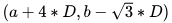](https://wiki.cept.org/uploads/images/gallery/2026-04/reVPRFJzws8i7Yw0-image.png),
where D is the inter-site distance.
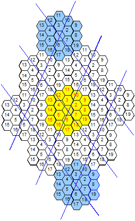
**Figure 185: Wrap-around with ’9’ clusters of 19 cells showing the toroidal nature of the wrap-around surface**
In the “ploting options” panel, you can toggle wrap-around plotting to allow easier selection of correct cell.