# 7.5 Cellular network positioning

# Introduction

5 panels characterised the positioning of a cellular system. This panel is the same whether a <span data-highlighted="true" data-vc="highlighted-text"><span class="_kqswh2mm"><span class="_5pioz8co _189e1dm9 _1il9buyh _19lc184f _d0altlke" data-testid="definition-highlighter">CDMA</span></span></span> (<span data-highlighted="true" data-vc="highlighted-text"><span class="_kqswh2mm"><span class="_5pioz8co _189e1dm9 _1il9buyh _19lc184f _d0altlke" data-testid="definition-highlighter">UL</span></span></span>/DL) or <span data-highlighted="true" data-vc="highlighted-text"><span class="_kqswh2mm"><span class="_5pioz8co _189e1dm9 _1il9buyh _19lc184f _d0altlke" data-testid="definition-highlighter">OFDMA</span></span></span> (<span data-highlighted="true" data-vc="highlighted-text">UL</span>/DL) is simulated.

[![image.png](https://wiki.cept.org/uploads/images/gallery/2026-04/scaled-1680-/VdQLXnkAxsI7rs5T-image.png)](https://wiki.cept.org/uploads/images/gallery/2026-04/VdQLXnkAxsI7rs5T-image.png)

# 7.5.1 System

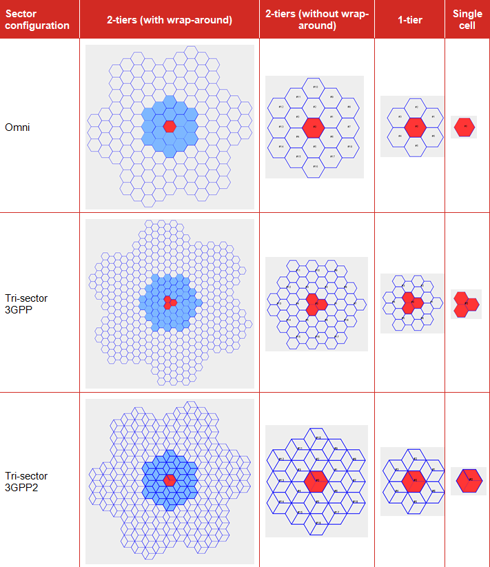
Initially macro-cellular environment was implemented in SEAMCAT, but with time more flexibility was given to the tool to reproduce various topology options in cellular network (Figure 176). Cell sites are laid out in a hexagonal grid. Sites with omni-directional antennas are placed in the middle of the cells as depicted in Figure 172 and sites with tri-sector antennas are placed at the edge of the cells, where each site covers three cells. Figure 173 shows one of these cell sites (small hexagons in dashed lines) and that the arrows demonstrate the antenna orientation of each cell. The BS to BS distance (also referred as inter-site distance in the literature) is D. The cell radius R is equal to *D/sqrt(3)* in the omni-antenna case and is equal to *D/3* in the tri-sector antenna case. Both suburban scenario and urban scenario can be modeled with this cell configuration. The scenarios differ only in propagation conditions and in the cell radius.

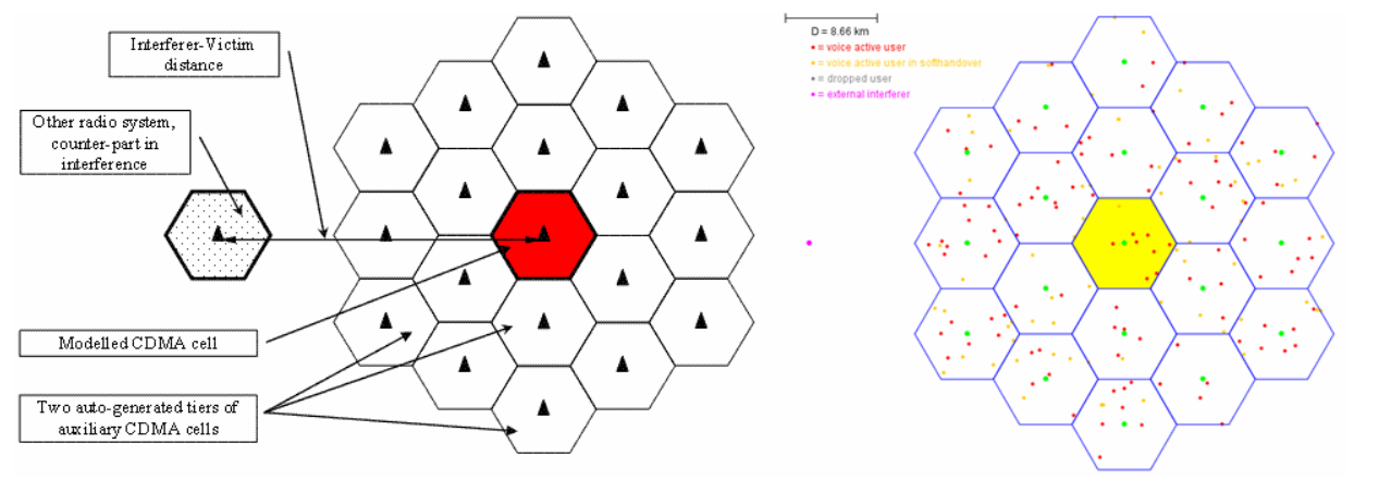
A wrap around cluster is used to reduce the number of cells required in the simulations and consequently to enable faster simulation run times. The number of cell sites in the cluster is assumed to be 19 (19 cells in the case of omnia-antenna and 57 cells in the case of tri-sector antenna), which appears to be appropriate for SEAMCAT simulation (see Section ‎7.6.3 for further details on wrap-around technique).

<table border="1" id="bkmrk-figure-172%3A-macro-ce" style="border-collapse: collapse; width: 100%;"><colgroup><col style="width: 50%;"></col><col style="width: 50%;"></col></colgroup><tbody><tr><td>[![image.png](https://wiki.cept.org/uploads/images/gallery/2026-04/scaled-1680-/BKxQ4kwoTkQ83RKw-image.png)](https://wiki.cept.org/uploads/images/gallery/2026-04/BKxQ4kwoTkQ83RKw-image.png)

</td><td>[![image.png](https://wiki.cept.org/uploads/images/gallery/2026-04/scaled-1680-/14mu3bGj7OqZkz7c-image.png)](https://wiki.cept.org/uploads/images/gallery/2026-04/14mu3bGj7OqZkz7c-image.png)

</td></tr><tr><td>**Figure 172: Macro-Cellular <span data-highlighted="true" data-vc="highlighted-text"><span class="_kqswh2mm"><span class="_5pioz8co _189e1dm9 _1il9buyh _19lc184f _d0altlke" data-testid="definition-highlighter">CDMA</span></span></span> Network Deployment with Omni Antenna**

</td><td>**Figure 173: Macro-Cellular <span data-highlighted="true" data-vc="highlighted-text">CDMA</span> Network Deployment with Tri-Sector Antenna**

</td></tr></tbody></table>

Therefore SEAMCAT supplements a single considered <span data-highlighted="true" data-vc="highlighted-text">CDMA</span> / <span data-highlighted="true" data-vc="highlighted-text"><span class="_kqswh2mm"><span class="_5pioz8co _189e1dm9 _1il9buyh _19lc184f _d0altlke" data-testid="definition-highlighter">OFDMA</span></span></span> cell with its Base Station (BS) two tiers of virtual cells to form a 19 cell (57 cell for tri-sector deployment) cluster, which is then populated with a certain number of mobile stations (MS) and a power control algorithm is then applied for balancing overall system, see Figure below:

[![image.png](https://wiki.cept.org/uploads/images/gallery/2026-04/scaled-1680-/IRGZHVQcR5FBDIuF-image.png)](https://wiki.cept.org/uploads/images/gallery/2026-04/IRGZHVQcR5FBDIuF-image.png)

**Figure 174: 19 cells omni setup**

<span data-highlighted="true" data-vc="highlighted-text">CDMA</span> and <span data-highlighted="true" data-vc="highlighted-text">OFDMA</span> module shares common platform like the positioning of the cellular layout. The celular topology in SEAMCAT is composed of the “Cell layout” and the “Cell radius”a shown in Figure 176.

In the “Cell Layout” you can select 2 tiers, 1 tier or single cell layout. In addition, you can select between Omni directional (single sector), tri-Sector (3GPP) and tri-Sector (3GPP2).

 The “Cell Radius” (km) is the size of the cell and defines also the BS to BS distance (i.e. inter-site distance).

[![image.png](https://wiki.cept.org/uploads/images/gallery/2026-04/scaled-1680-/bwEpakOakP0ZrYId-image.png)](https://wiki.cept.org/uploads/images/gallery/2026-04/bwEpakOakP0ZrYId-image.png)

**Figure 176: Overview of the topology options in cellular network**

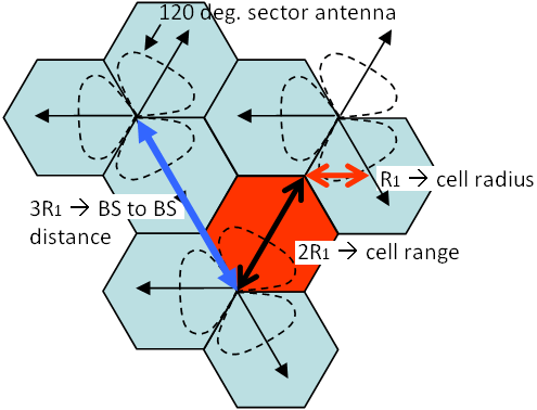
Two types of hexagonal grids are used to represent cellular layout, there is the 3GPP ([http://www.3gpp.org/](http://www.3gpp.org/ "http://www.3gpp.org/")) and the 3GPP2 ([http://www.3gpp2.org/](http://www.3gpp2.org/ "http://www.3gpp2.org/")). The differences are illustrated in Figure 177 (3GPP) and in Figure 178 (3GPP2). The fundamental principal of the two approaches is that they share the same commonality for the BS to BS. Based on this same value, it is possible to extract the relationship of the cell range and cell radius between the two approaches.

Within the <span data-highlighted="true" data-vc="highlighted-text"><span class="_kqswh2mm"><span class="_5pioz8co _189e1dm9 _1il9buyh _19lc184f _d0altlke" data-testid="definition-highlighter">CEPT</span></span></span> work, it is more common to use the 3GPP hexagonal grid, <span data-highlighted="true" data-vc="highlighted-text"><span class="_kqswh2mm"><span class="_5pioz8co _189e1dm9 _1il9buyh _19lc184f _d0altlke" data-testid="definition-highlighter">ECC</span></span></span> Repport 82 ‎\[6\] and <span data-highlighted="true" data-vc="highlighted-text">ECC</span> Repport 96 ‎\[7\].

Figure 177 presents an example of the 3GPP approach:

[![image.png](https://wiki.cept.org/uploads/images/gallery/2026-04/scaled-1680-/3lmOUtrGVce3tgfx-image.png)](https://wiki.cept.org/uploads/images/gallery/2026-04/3lmOUtrGVce3tgfx-image.png)

**Figure 177: 3GPP illustration of the Cell Radius, Cell Range and BS to BS distance**

<div class="pm-table-container with-shadow-observer" data-layout="align-start" data-testid="table-container" id="bkmrk-where%3A-cell-radius-%3D"><div class="pm-table-sticky-scrollbar-sentinel-top" data-testid="sticky-scrollbar-sentinel-top">  
</div><div class="pm-table-wrapper" data-autosize="false" data-layout="align-start" data-number-column="false" data-table-local-id="" data-vc="table-node-wrapper"><div class="sentinel-left">  
</div><table data-layout="align-start" data-number-column="false" data-table-width="760" data-testid="renderer-table" style="width: 100%;"><colgroup><col style="width: 26.3346%;"></col><col style="width: 36.8208%;"></col><col style="width: 36.8208%;"></col></colgroup><tbody><tr><td style="width: 26.3605%;">where:

</td><td style="width: 36.7772%;">Cell Radius = R<sub data-renderer-mark="true">1</sub>

Cell Range = 2R<sub data-renderer-mark="true">1</sub>

BS to BS distance = 3R<sub data-renderer-mark="true">1</sub>

</td><td style="width: 36.7772%;">(Eq.31)

</td></tr></tbody></table>

<div class="sentinel-right">  
</div></div></div>What is important is that the BS to BS station distance be the same between the 3GPP and the 3GPP2 approach, i.e. where 3R<sub data-renderer-mark="true">1 </sub>= 2h which is equivalent to R = sqrt(3) R<sub data-renderer-mark="true">1</sub>.

From there it is possible to extract the cell radius in SEAMCAT.

**Table 21: Example of the distances relationship between 3GPP and SEAMCAT**

<div class="pm-table-container with-shadow-observer" data-layout="align-start" data-testid="table-container" id="bkmrk-%C2%A0-urban-case-rural-c"><div class="pm-table-wrapper" data-autosize="false" data-layout="align-start" data-number-column="false" data-table-local-id="" data-vc="table-node-wrapper"><div class="sentinel-right"><div class="pm-table-container with-shadow-observer" data-layout="align-start" data-testid="table-container"><div class="pm-table-wrapper" data-autosize="false" data-layout="align-start" data-number-column="false" data-table-local-id="" data-vc="table-node-wrapper"><table data-layout="align-start" data-number-column="false" data-table-width="760" data-testid="renderer-table" style="width: 107.619%;"><tbody><tr><td colspan="1" rowspan="1" style="width: 49.758%;"></td><td colspan="1" rowspan="1" style="width: 28.2819%;">**Urban Case**

</td><td colspan="1" rowspan="1" style="width: 21.9298%;">**Rural Case**

</td></tr><tr><td colspan="1" rowspan="1" style="width: 49.758%;">SEAMCAT cell radius (R)=

</td><td colspan="1" rowspan="1" style="width: 28.2819%;">433 m

</td><td colspan="1" rowspan="1" style="width: 21.9298%;">4330 m

</td></tr><tr><td colspan="1" rowspan="1" style="width: 49.758%;">SEAMCAT cell range (h)=

</td><td colspan="1" rowspan="1" style="width: 28.2819%;">375 m

</td><td colspan="1" rowspan="1" style="width: 21.9298%;">3750 m

</td></tr><tr><td colspan="1" rowspan="1" style="width: 49.758%;">Distance BS to BS (2h = 3 R<sub data-renderer-mark="true">1</sub>) =

</td><td colspan="1" rowspan="1" style="width: 28.2819%;">750 m

</td><td colspan="1" rowspan="1" style="width: 21.9298%;">7500 m

</td></tr><tr><td colspan="1" rowspan="1" style="width: 49.758%;">3GPP cell range (2R<sub data-renderer-mark="true">1</sub>) =

</td><td colspan="1" rowspan="1" style="width: 28.2819%;">500 m

</td><td colspan="1" rowspan="1" style="width: 21.9298%;">5000 m

</td></tr><tr><td colspan="1" rowspan="1" style="width: 49.758%;">3GPP cell radius (R<sub data-renderer-mark="true">1</sub>) =

</td><td colspan="1" rowspan="1" style="width: 28.2819%;">250 m

</td><td colspan="1" rowspan="1" style="width: 21.9298%;">2500 m

</td></tr></tbody></table>

</div><div class="sentinel-right">  
</div></div></div></div></div>In summary, according to Figure 179 below, the Table 22 shows the current different definitions for sector, cell and radii:

<div class="pm-table-container with-shadow-observer" data-layout="align-start" data-testid="table-container" id="bkmrk-table-22%3A-different-"><div class="pm-table-wrapper" data-autosize="false" data-layout="align-start" data-number-column="false" data-table-local-id="" data-vc="table-node-wrapper"><div class="sentinel-right"><div class="pm-table-container with-shadow-observer" data-layout="align-start" data-testid="table-container"><div class="sentinel-right"><div class="fabric-editor-block-mark fabric-editor-alignment align-center" data-align="center">**Table 22: Different definitions for sector, cell and radii**</div></div></div></div></div></div><div class="pm-table-container with-shadow-observer" data-layout="align-start" data-testid="table-container" id="bkmrk-parameter-3gpp-tr-36"><div class="pm-table-wrapper" data-autosize="false" data-layout="align-start" data-number-column="false" data-table-local-id="" data-vc="table-node-wrapper"><div class="sentinel-right"><div class="pm-table-container with-shadow-observer" data-layout="align-start" data-testid="table-container"><div class="sentinel-right"><div class="pm-table-container with-shadow-observer" data-layout="align-start" data-testid="table-container"><div class="pm-table-wrapper" data-autosize="false" data-layout="align-start" data-number-column="false" data-table-local-id="" data-vc="table-node-wrapper"><table data-layout="align-start" data-number-column="false" data-table-width="760" data-testid="renderer-table" style="width: 108.333%;"><colgroup></colgroup><tbody><tr><td colspan="1" rowspan="1" style="width: 19.4787%;">**Parameter**

</td><td colspan="1" rowspan="1" style="width: 18.4761%;">**3GPP <span data-highlighted="true" data-vc="highlighted-text"><span class="_kqswh2mm"><span class="_5pioz8co _189e1dm9 _1il9buyh _19lc184f _d0altlke" data-testid="definition-highlighter">TR</span></span></span> 36.942**

</td><td colspan="1" rowspan="1" style="width: 28.9315%;">**<span data-highlighted="true" data-vc="highlighted-text">ECC</span> Report 252 and others**

</td><td colspan="1" rowspan="1" style="width: 33.0851%;">**Recommendation <span data-highlighted="true" data-vc="highlighted-text"><span class="_kqswh2mm"><span class="_5pioz8co _189e1dm9 _1il9buyh _19lc184f _d0altlke" data-testid="definition-highlighter">ITU-R</span></span></span> M.2101**

**Report <span data-highlighted="true" data-vc="highlighted-text">ITU-R</span> M.2292**

</td></tr><tr><td colspan="1" rowspan="1" style="width: 19.4787%;">**Sector**

</td><td colspan="1" rowspan="1" style="width: 18.4761%;">1 hexagon

</td><td colspan="1" rowspan="1" style="width: 28.9315%;">1 hexagon

</td><td colspan="1" rowspan="1" style="width: 33.0851%;">1 hexagon

</td></tr><tr><td colspan="1" rowspan="1" style="width: 19.4787%;">**Cell**

</td><td colspan="1" rowspan="1" style="width: 18.4761%;">3 hexagon

</td><td colspan="1" rowspan="1" style="width: 28.9315%;">3 hexagon

</td><td colspan="1" rowspan="1" style="width: 33.0851%;">1 hexagon

</td></tr><tr><td colspan="1" rowspan="1" style="width: 19.4787%;">**Cell radius**

</td><td colspan="1" rowspan="1" style="width: 18.4761%;">X

</td><td colspan="1" rowspan="1" style="width: 28.9315%;">X

</td><td colspan="1" rowspan="1" style="width: 33.0851%;">Y = 2\*X

</td></tr><tr><td colspan="1" rowspan="1" style="width: 19.4787%;">**Cell range**

</td><td colspan="1" rowspan="1" style="width: 18.4761%;">Y = 2\*X

</td><td colspan="1" rowspan="1" style="width: 28.9315%;">Y = 2\*X

</td><td colspan="1" rowspan="1" style="width: 33.0851%;">Not defined

</td></tr><tr><td colspan="1" rowspan="1" style="width: 19.4787%;">**BS to BS distance**

</td><td colspan="1" rowspan="1" style="width: 18.4761%;">Z = 3\*X

</td><td colspan="1" rowspan="1" style="width: 28.9315%;">Z = 3\*X

</td><td colspan="1" rowspan="1" style="width: 33.0851%;">Z = 3\*X

</td></tr></tbody></table>

<div class="sentinel-right">  
</div></div><div class="pm-table-sticky-scrollbar-container-view-page" data-vc="table-sticky-scrollbar-container"><div>  
</div></div><div class="pm-table-sticky-scrollbar-sentinel-bottom" data-testid="sticky-scrollbar-sentinel-bottom">  
</div></div></div></div></div></div></div>[![image.png](https://wiki.cept.org/uploads/images/gallery/2026-04/scaled-1680-/QcznPW01FfHVo8Ub-image.png)](https://wiki.cept.org/uploads/images/gallery/2026-04/QcznPW01FfHVo8Ub-image.png)

Figure 179: Different definitions for sector, cell and radii

<div class="pm-table-container with-shadow-observer" data-layout="align-start" data-testid="table-container" id="bkmrk--5"><div class="pm-table-wrapper" data-autosize="false" data-layout="align-start" data-number-column="false" data-table-local-id="" data-vc="table-node-wrapper"><div class="sentinel-right"><div class="pm-table-container with-shadow-observer" data-layout="align-start" data-testid="table-container"><div class="sentinel-right"><div class="pm-table-container with-shadow-observer" data-layout="align-start" data-testid="table-container"><div class="pm-table-sticky-scrollbar-sentinel-bottom" data-testid="sticky-scrollbar-sentinel-bottom">  
</div></div></div></div></div></div></div><div class="pm-table-container with-shadow-observer" data-layout="align-start" data-testid="table-container" id="bkmrk--6"><div class="pm-table-wrapper" data-autosize="false" data-layout="align-start" data-number-column="false" data-table-local-id="" data-vc="table-node-wrapper"><div class="sentinel-right"><div class="pm-table-container with-shadow-observer" data-layout="align-start" data-testid="table-container"><div class="sentinel-right">  
</div><div class="pm-table-sticky-scrollbar-container-view-page" data-vc="table-sticky-scrollbar-container"><div>  
</div></div><div class="pm-table-sticky-scrollbar-sentinel-bottom" data-testid="sticky-scrollbar-sentinel-bottom">  
</div></div></div></div></div><div class="pm-table-container with-shadow-observer" data-layout="align-start" data-testid="table-container" id="bkmrk--7"><div class="pm-table-wrapper" data-autosize="false" data-layout="align-start" data-number-column="false" data-table-local-id="" data-vc="table-node-wrapper"><div class="sentinel-right">  
</div></div><div class="pm-table-sticky-scrollbar-container-view-page" data-vc="table-sticky-scrollbar-container"><div>  
</div></div><div class="pm-table-sticky-scrollbar-sentinel-bottom" data-testid="sticky-scrollbar-sentinel-bottom">  
</div></div>

# 7.5.2 System layout - reference cell selection

A singe cell consists of several MSs connected to their serving <span data-highlighted="true" data-vc="highlighted-text"><span class="_kqswh2mm"><span class="_5pioz8co _189e1dm9 _1il9buyh _19lc184f _d0altlke" data-testid="definition-highlighter">BS</span></span></span>. The reference cell is a single cell that is surrounded by two tiers of virtual cells to form a 19 cells (or 57 cells for tri-sector deployment) cluster. This cells clutter is then populated with a certain number of MSs. The reference cell is by default at the center of the network, but you can modify it by selecting any cells you want. Part of configuring a <span data-highlighted="true" data-vc="highlighted-text"><span class="_kqswh2mm"><span class="_5pioz8co _189e1dm9 _1il9buyh _19lc184f _d0altlke" data-testid="definition-highlighter">CDMA</span></span></span> or <span data-highlighted="true" data-vc="highlighted-text"><span class="_kqswh2mm"><span class="_5pioz8co _189e1dm9 _1il9buyh _19lc184f _d0altlke" data-testid="definition-highlighter">OFDMA</span></span></span> network is selecting the reference cell. In SEAMCAT it is possible to choose between two network configurations (3GPP and 3GPP2, see Figure 176).

The reference cell in Figure 180 is used to calculate the effects of interference and to measure results and all non reference cells are used to provide a proper interference background to the reference cell. You can click on the cell that should be used as reference cell when gathering results. The red cell is the current selection.

![image.png](https://wiki.cept.org/uploads/images/gallery/2026-04/scaled-1680-/149Xz7xO16ez95Gn-image.png)

**Figure 180: System layout - reference cell selection**

<div class="fabric-editor-block-mark fabric-editor-alignment align-center" data-align="center" id="bkmrk-table-23%3A-system-lay"><div class="inline-extension-renderer css-e2q2ep"><span class="css-6k4g17">  
</span></div>**Table 23: System layout GUI**</div><div class="fabric-editor-block-mark fabric-editor-alignment align-center" data-align="center" id="bkmrk--1"></div><div class="pm-table-container with-shadow-observer" data-layout="align-start" data-testid="table-container" id="bkmrk-description-symbol-t"><div class="pm-table-wrapper" data-autosize="false" data-layout="align-start" data-number-column="false" data-table-local-id="" data-vc="table-node-wrapper"><table data-layout="align-start" data-number-column="false" data-table-width="760" data-testid="renderer-table" style="width: 100%;"><colgroup></colgroup><tbody><tr><td colspan="1" rowspan="1" style="width: 20.2574%;">**Description**

</td><td colspan="1" rowspan="1" style="width: 5.95806%;">**Symbol**

</td><td colspan="1" rowspan="1" style="width: 9.64853%;">**Type**

</td><td colspan="1" rowspan="1" style="width: 5.24661%;">**Unit**

</td><td colspan="1" rowspan="1" style="width: 58.8656%;">**Comments**

</td></tr><tr><td colspan="1" rowspan="1" style="width: 20.2574%;">**Center of infinite network**

</td><td colspan="1" rowspan="1" style="width: 5.95806%;">-

</td><td colspan="1" rowspan="1" style="width: 9.64853%;">Boolean

</td><td colspan="1" rowspan="1" style="width: 5.24661%;">-

</td><td colspan="1" rowspan="1" style="width: 58.8656%;">Quick access to predefined selection of reference cell. This only changes the selected reference cell – no other simulation parameter is changed.

</td></tr><tr><td colspan="1" rowspan="1" style="width: 20.2574%;">**Left hand side of network**

</td><td colspan="1" rowspan="1" style="width: 5.95806%;">-

</td><td colspan="1" rowspan="1" style="width: 9.64853%;">Boolean

</td><td colspan="1" rowspan="1" style="width: 5.24661%;">-

</td><td colspan="1" rowspan="1" style="width: 58.8656%;">Position the reference cell on the left hand side of the network. Can be used to reproduce border network layout.

</td></tr><tr><td colspan="1" rowspan="1" style="width: 20.2574%;">**Right hand side of network**

</td><td colspan="1" rowspan="1" style="width: 5.95806%;">-

</td><td colspan="1" rowspan="1" style="width: 9.64853%;">Boolean

</td><td colspan="1" rowspan="1" style="width: 5.24661%;">-

</td><td colspan="1" rowspan="1" style="width: 58.8656%;">Position the reference cell on the right hand side of the network. Can be used to reproduce border network layout.

</td></tr><tr><td colspan="1" rowspan="1" style="width: 20.2574%;">**Measure interference from entire cluster**

</td><td colspan="1" rowspan="1" style="width: 5.95806%;">-

</td><td colspan="1" rowspan="1" style="width: 9.64853%;">Boolean

</td><td colspan="1" rowspan="1" style="width: 5.24661%;">-

</td><td colspan="1" rowspan="1" style="width: 58.8656%;">See section ‎7.6.2

</td></tr><tr><td colspan="1" rowspan="1" style="width: 20.2574%;">**Generate wrap-around**

</td><td colspan="1" rowspan="1" style="width: 5.95806%;">-

</td><td colspan="1" rowspan="1" style="width: 9.64853%;">Boolean

</td><td colspan="1" rowspan="1" style="width: 5.24661%;">-

</td><td colspan="1" rowspan="1" style="width: 58.8656%;">See section ‎7.6.3

</td></tr></tbody></table>

<div class="sentinel-right">  
</div></div><div class="pm-table-sticky-scrollbar-container-view-page" data-vc="table-sticky-scrollbar-container"><div>  
</div></div><div class="pm-table-sticky-scrollbar-sentinel-bottom" data-testid="sticky-scrollbar-sentinel-bottom">Normally the considered cellular system (<span data-highlighted="true" data-vc="highlighted-text">CDMA</span> or <span data-highlighted="true" data-vc="highlighted-text">OFDMA</span>) is modelled as endless network using the so called wrap-around technique. Alternatively, you may specify that the modelled cellular cell is laying at the edge of the network, in this case the cellular system will be modelled as if extending to one side only. The latter case may be suitable for simulation of geographically separated victim and interfering systems, like in cross-border scenarios as illustrated in Figure 181. </div><div class="pm-table-sticky-scrollbar-sentinel-bottom" data-testid="sticky-scrollbar-sentinel-bottom"></div></div>[![image.png](https://wiki.cept.org/uploads/images/gallery/2026-04/scaled-1680-/kuOLdibMOGhbfHwG-image.png)](https://wiki.cept.org/uploads/images/gallery/2026-04/kuOLdibMOGhbfHwG-image.png)

[![image.png](https://wiki.cept.org/uploads/images/gallery/2026-04/scaled-1680-/HekFh3o2A862wPWr-image.png)](https://wiki.cept.org/uploads/images/gallery/2026-04/HekFh3o2A862wPWr-image.png)

[![image.png](https://wiki.cept.org/uploads/images/gallery/2026-04/scaled-1680-/r9WsliKAcl8hWDDF-image.png)](https://wiki.cept.org/uploads/images/gallery/2026-04/r9WsliKAcl8hWDDF-image.png)

 **Figure 181: Example on how to set up the system layout to reproduce a border coordination scenario**

# 7.5.3 System layout preview

You have the possibility to see a preview of the network you are simulating. You can click on the cell that should be used as reference cell when gathering results. The red cell is the current selection.

[![image.png](https://wiki.cept.org/uploads/images/gallery/2026-04/scaled-1680-/3oYrWvnYdP3QCzgN-image.png)](https://wiki.cept.org/uploads/images/gallery/2026-04/3oYrWvnYdP3QCzgN-image.png)

<div class="rich-media-item mediaSingleView-content-wrap image-align-start css-tvrmtx" data-layout="align-start" data-media-vc-wrapper="true" data-node-type="mediaSingle" data-renderer-start-pos="208" data-vc="media-single" data-width="345" data-width-type="pixel" id="bkmrk--1"><div class="css-47n9kv"><div data-alt="" data-collection="contentId-494388" data-context-id="494388" data-file-mime-type="" data-file-name="file" data-file-size="1" data-height="433" data-id="f41c9435-bf66-455e-a54b-32ea34926e52" data-node-type="media" data-renderer-start-pos="209" data-type="file" data-width="598"><div class="_2rko18qm _vchhusvi _kqswh2mm _ect4ttxp _p12f1osq _c71l1osq _1bsb1qmm _4t3ine4n _1hlmd0i9 _1rquusvi _eg541i5c _mts3kb7n _1ntskb7n _yfmhtlke _5sb1v00u new-file-experience-wrapper" data-media-vc-wrapper="true" data-testid="media-card-view" id="bkmrk--2"><div class="_1reo15vq _18m915vq _2rko18qm _1e0c1txw _kqswh2mm _p12f1osq _1bsb1osq _4t3i1osq _c71l1osq media-file-card-view" data-cursor="pointer" data-test-media-name="82.png" data-test-progress="1" data-test-source="remote" data-test-status="complete" data-testid="media-file-card-view"><div class="_kqswstnw _1bsb1osq _4t3i1osq _1e0c1txw _2lx21bp4 _1bah1h6o _4cvr1h6o" data-testid="ImageRendererWrapper">![](blob:https://ecowiki.atlassian.net/ae4ff7d8-c3c9-4ce5-8fd9-30e0c6afb810#media-blob-url=true&id=f41c9435-bf66-455e-a54b-32ea34926e52&collection=contentId-494388&contextId=494388&width=598&height=433&alt=&clientId=113268fe-fe5b-4bc3-8ff3-07965dbf1d18)</div></div></div></div></div></div><div class="fabric-editor-block-mark fabric-editor-alignment align-center" data-align="center" id="bkmrk-figure-182%3A-system-l">**Figure 182: System layout preview**</div>

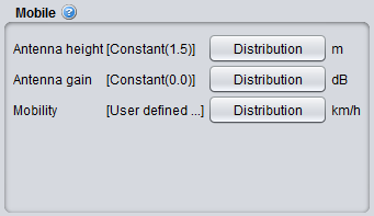
# 7.5.4 Mobile station

[![image.png](https://wiki.cept.org/uploads/images/gallery/2026-04/scaled-1680-/nGuOZ5jGU7ViGMdN-image.png)](https://wiki.cept.org/uploads/images/gallery/2026-04/nGuOZ5jGU7ViGMdN-image.png)

**Figure 183: Cellular system – Mobile station GUI**

<div class="fabric-editor-block-mark fabric-editor-alignment align-center" data-align="center" id="bkmrk-table-24%3A-cellular-s"><div class="inline-extension-renderer css-e2q2ep"><span class="css-6k4g17">  
</span></div>**Table 24: Cellular system – Mobile station parameters**</div><div class="fabric-editor-block-mark fabric-editor-alignment align-center" data-align="center" id="bkmrk--1"></div><div class="pm-table-container with-shadow-observer" data-layout="align-start" data-testid="table-container" id="bkmrk-description-symbol-t"><div class="pm-table-wrapper" data-autosize="false" data-layout="align-start" data-number-column="false" data-table-local-id="" data-vc="table-node-wrapper"><table data-layout="align-start" data-number-column="false" data-table-width="760" data-testid="renderer-table" style="width: 100%;"><colgroup></colgroup><tbody><tr><td colspan="1" rowspan="1" style="width: 16.9209%;">**Description**

</td><td colspan="1" rowspan="1" style="width: 9.17404%;">**Symbol**

</td><td colspan="1" rowspan="1" style="width: 21.212%;">**Type**

</td><td colspan="1" rowspan="1" style="width: 10.367%;">**Unit**

</td><td colspan="1" rowspan="1" style="width: 42.3022%;">**Comments**

</td></tr><tr><td colspan="1" rowspan="1" style="width: 16.9209%;">**Antenna height**

</td><td colspan="1" rowspan="1" style="width: 9.17404%;">H<sub data-renderer-mark="true">MS</sub>

</td><td colspan="1" rowspan="1" style="width: 21.212%;">Distribution or Scalar

</td><td colspan="1" rowspan="1" style="width: 10.367%;">m

</td><td colspan="1" rowspan="1" style="width: 42.3022%;">Height of user terminal in meters. Note that the assumed antenna height definition (above ground, above local clutter, effective antenna height) should correspond to the selected propagation model.

</td></tr><tr><td colspan="1" rowspan="1" style="width: 16.9209%;">**Antenna gain**

</td><td colspan="1" rowspan="1" style="width: 9.17404%;">G<sub data-renderer-mark="true">Tx</sub> , G<sub data-renderer-mark="true">Tx</sub>

</td><td colspan="1" rowspan="1" style="width: 21.212%;">Distribution or Scalar

</td><td colspan="1" rowspan="1" style="width: 10.367%;">dB

</td><td colspan="1" rowspan="1" style="width: 42.3022%;">An omni directional antenna pattern is assumed. Depending on the link direction, it can be either the gain of the Tx (<span data-highlighted="true" data-vc="highlighted-text"><span class="_kqswh2mm"><span class="_5pioz8co _189e1dm9 _1il9buyh _19lc184f _d0altlke" data-testid="definition-highlighter">UL</span></span></span>) or the Rx (DL)

</td></tr><tr><td colspan="1" rowspan="1" style="width: 16.9209%;">**Mobility**

</td><td colspan="1" rowspan="1" style="width: 9.17404%;">-

</td><td colspan="1" rowspan="1" style="width: 21.212%;">Distribution or Scalar

</td><td colspan="1" rowspan="1" style="width: 10.367%;">Km/h

</td><td colspan="1" rowspan="1" style="width: 42.3022%;">Distribution of speed among the users.Theese speeds have to conform to the speed options in the selected Link Level Data (Section 8.5).

For simplicity SEAMCAT assumes four different speeds, assigned to mobile users with uniform probability:

- 0 km/h - No movement,
- 3 km/h - Walking,
- 30 km/h - Urban driving,

100 km/h - Motorway driving

</td></tr></tbody></table>

<div class="sentinel-right">  
</div></div><div class="pm-table-sticky-scrollbar-container-view-page" data-vc="table-sticky-scrollbar-container"><div>  
</div></div><div class="pm-table-sticky-scrollbar-sentinel-bottom" data-testid="sticky-scrollbar-sentinel-bottom">  
</div></div>

# 7.5.5 Base station

[![image.png](https://wiki.cept.org/uploads/images/gallery/2026-04/scaled-1680-/XWUkhfaObgt2ibjD-image.png)](https://wiki.cept.org/uploads/images/gallery/2026-04/XWUkhfaObgt2ibjD-image.png)

**Figure 184: Cellular system – Base station GUI**

<div class="fabric-editor-block-mark fabric-editor-alignment align-center" data-align="center" id="bkmrk-table-25%3A-cellular-s"><div class="inline-extension-renderer css-e2q2ep"><span class="css-6k4g17">  
</span></div>**Table 25: Cellular system – Base station parameters**</div><div class="fabric-editor-block-mark fabric-editor-alignment align-center" data-align="center" id="bkmrk--1"></div><div class="pm-table-container with-shadow-observer" data-layout="align-start" data-testid="table-container" id="bkmrk-description-symbol-t"><div class="pm-table-wrapper" data-autosize="false" data-layout="align-start" data-number-column="false" data-table-local-id="" data-vc="table-node-wrapper"><table data-layout="align-start" data-number-column="false" data-table-width="760" data-testid="renderer-table" style="width: 100%;"><colgroup></colgroup><tbody><tr><td colspan="1" rowspan="1" style="width: 12.2736%;">**Description**

</td><td colspan="1" rowspan="1" style="width: 6.91134%;">**Symbol**

</td><td colspan="1" rowspan="1" style="width: 24.4085%;">**Type**

</td><td colspan="1" rowspan="1" style="width: 16.8212%;">**Unit**

</td><td colspan="1" rowspan="1" style="width: 39.5615%;">**Comments**

</td></tr><tr><td colspan="1" rowspan="1" style="width: 12.2736%;">Antenna height

</td><td colspan="1" rowspan="1" style="width: 6.91134%;">H<sub data-renderer-mark="true"><span data-highlighted="true" data-vc="highlighted-text"><span class="_kqswh2mm"><span class="_5pioz8co _189e1dm9 _1il9buyh _19lc184f _d0altlke" data-testid="definition-highlighter">BS</span></span></span></sub>

</td><td colspan="1" rowspan="1" style="width: 24.4085%;">Distribution or Scalar

</td><td colspan="1" rowspan="1" style="width: 16.8212%;">m

</td><td colspan="1" rowspan="1" style="width: 39.5615%;">Distribution used to determine height of <span data-highlighted="true" data-vc="highlighted-text">BS</span>. Note that the assumed antenna height definition (above ground, above local clutter, effective antenna height) should correspond to the selected propagation model

</td></tr><tr><td colspan="1" rowspan="1" style="width: 12.2736%;">Antenna tilt

</td><td colspan="1" rowspan="1" style="width: 6.91134%;">-

</td><td colspan="1" rowspan="1" style="width: 24.4085%;">Distribution or Scalar

</td><td colspan="1" rowspan="1" style="width: 16.8212%;">degree

</td><td colspan="1" rowspan="1" style="width: 39.5615%;">Equivalent to a physical tilt of an antenna on a mast, (-) sign is a downtilt, (+) sign is an uptilt. See **‎**ANNEX 11: for further details and illustration.

</td></tr><tr><td colspan="1" rowspan="1" style="width: 12.2736%;">Antenna pattern

</td><td colspan="1" rowspan="1" style="width: 6.91134%;">-

</td><td colspan="1" rowspan="1" style="width: 24.4085%;">Library

</td><td colspan="1" rowspan="1" style="width: 16.8212%;">-

</td><td colspan="1" rowspan="1" style="width: 39.5615%;">See Section **‎**5.2.3

</td></tr></tbody></table>

<div class="sentinel-right">  
</div></div><div class="pm-table-sticky-scrollbar-container-view-page" data-vc="table-sticky-scrollbar-container"><div>  
</div></div><div class="pm-table-sticky-scrollbar-sentinel-bottom" data-testid="sticky-scrollbar-sentinel-bottom">  
</div></div>