| **Description** | **Symbol** | **Type** | **Unit** | **Comments** |
| Interferer is CR | switch | When the CR button is checked then it allows to set the emission characteristics of the VLT (used for the sRSS calculation only) | ||
| Emission mask: Unwanted signal level (VLT) | Function (X,Y) (MHz) | dBm/reference bandw. (MHz) | Define the mask of the transmitter, in the emission bandwidth and out of the emission bandwidth. Negative values in the relative mask should be chosen in a way that the integration over the emission bandwidth results in the total emitted power. If constant mask, there is no emission outside of the bandwidth. | |
| Unwanted emissions floor: Noise floor signal level | Function (X,Y) (MHz) | dBm/ reference bandw. (MHz) | Define the minimum strength of the unwanted emissions. So the unwanted emissions equal to Max(Pwt + Unwanted emission, Unwanted emissions floor) |
| [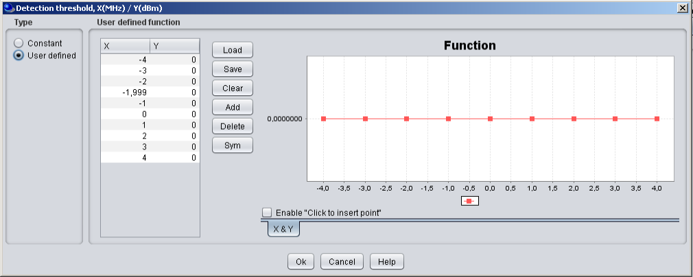](https://wiki.cept.org/uploads/images/gallery/2026-04/NvsnjPbEqoFTFgHm-image.png) | [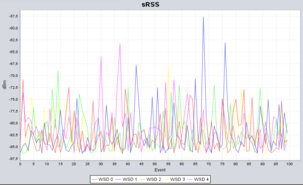](https://wiki.cept.org/uploads/images/gallery/2026-04/7br9kXHluPxleAh6-image.png) |
| **Figure 160: Selection of a high** **detection threshold** | **Figure 161: The sRSS values are well below the** **detection threshold, so no victim system have been detected** |
| [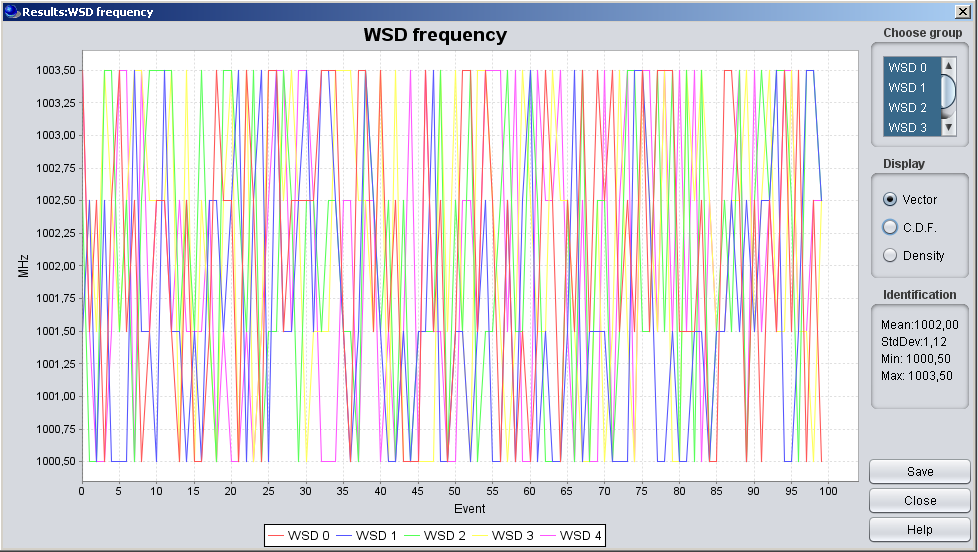](https://wiki.cept.org/uploads/images/gallery/2026-04/uKImCZtBjBA3mh3a-image.png) | [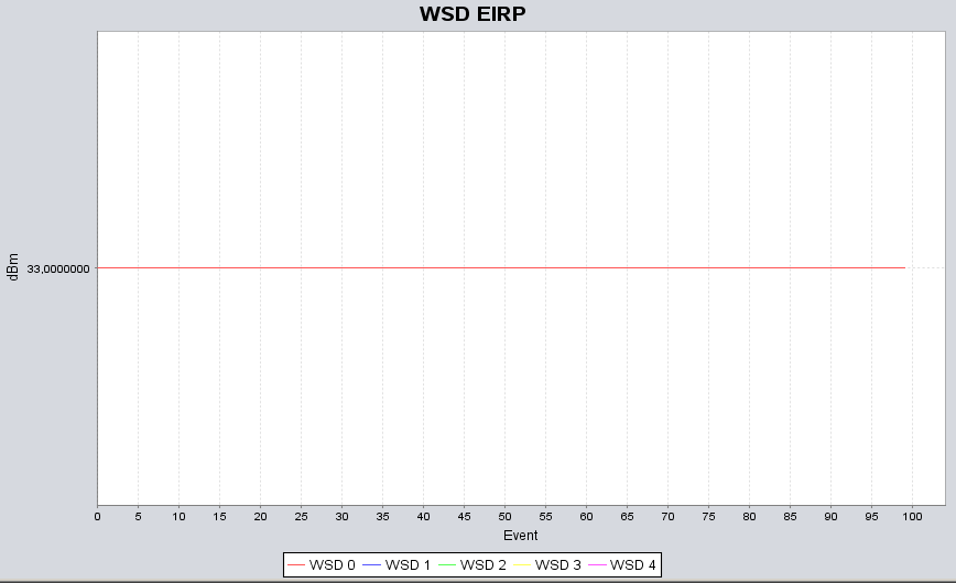](https://wiki.cept.org/uploads/images/gallery/2026-04/1oGjqenBp7CqIXsK-image.png) |
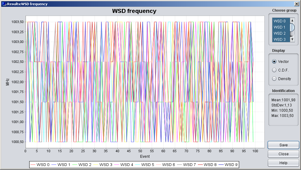
| **Figure 162: The WSD can transmit anywhere** **in the victim frequency range** | **Figure 163: e.i.r.p. set to -33 dBm as set in the It, i.e.** **Txpower (=-33 dBm) + Gmax (=0 dBi),** **meaning that there were no limit applied to the It Tx power** |
| [](https://wiki.cept.org/uploads/images/gallery/2026-04/h74WnMtwgom9jRoR-image.png) | [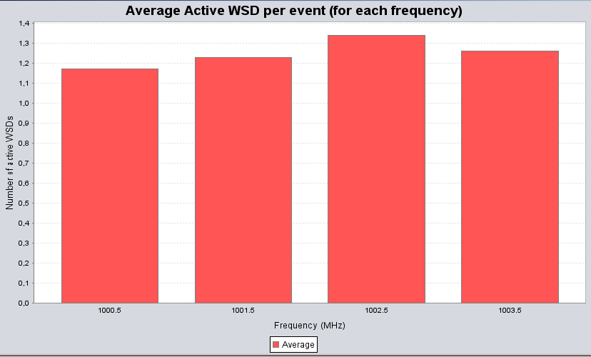](https://wiki.cept.org/uploads/images/gallery/2026-04/jvK756FGpTw2lHV8-image.png) |
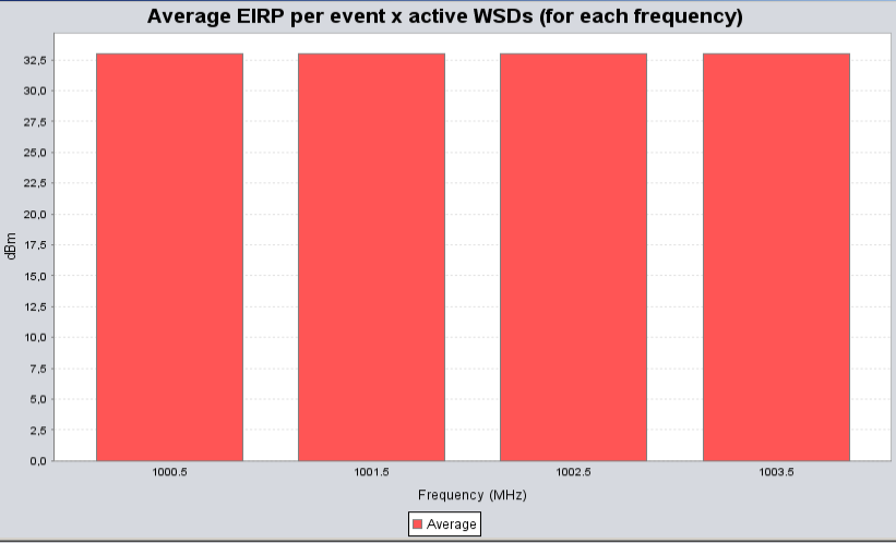
| **Figure 164: e.i.r.p. is the same irrespective of the frequency** | **Figure 165: Illustration of the number of WSDs per frequency** |
| [](https://wiki.cept.org/uploads/images/gallery/2026-04/eoWBw1VczAacfQXx-image.png) | [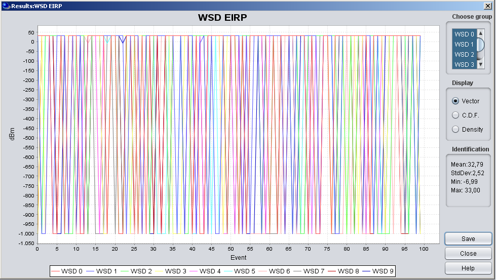](https://wiki.cept.org/uploads/images/gallery/2026-04/0cw7Dr7SuQQAFmnz-image.png) |
| **(a) WSD frequency** | **(b) WSD e.i.r.p.** |
| [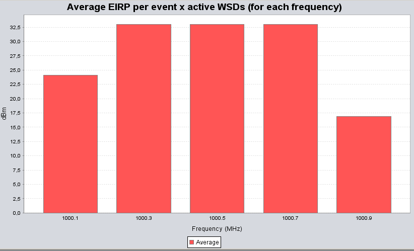](https://wiki.cept.org/uploads/images/gallery/2026-04/MY0UAVVeYzGuJbHR-image.png) | [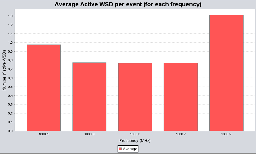](https://wiki.cept.org/uploads/images/gallery/2026-04/L311iPSAU3O6TW8E-image.png) |
| **(a) average e.i.r.p.** | **(b) average number of active WSDs** |