6.5 Examples

• 6.5.1 All the channels are available
• 6.5.2 All the channels are blocked
• 6.5.3 Some of the channels are blocked and some are available

6.5.1 All the channels are available

 

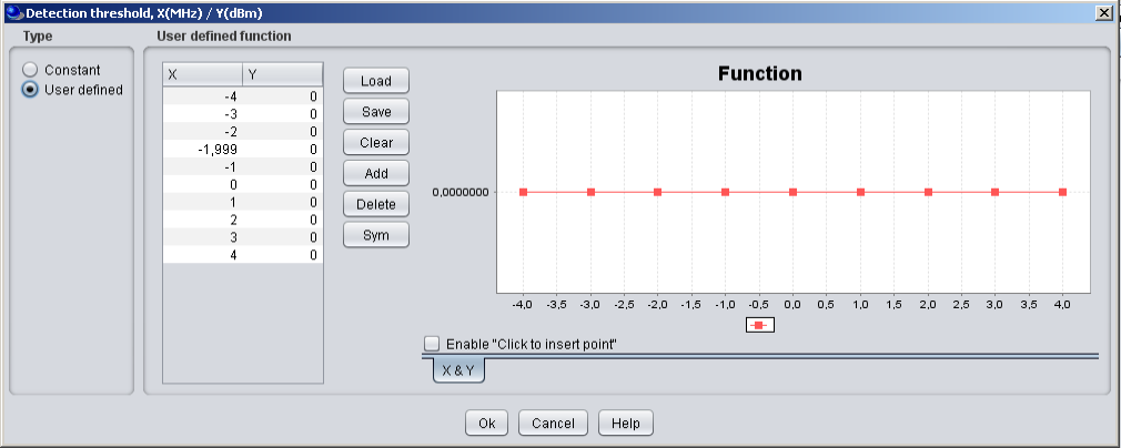
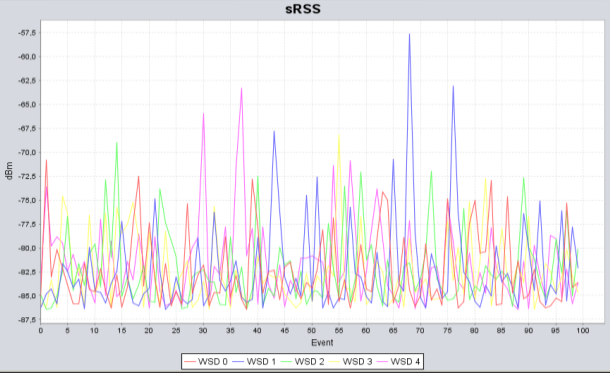
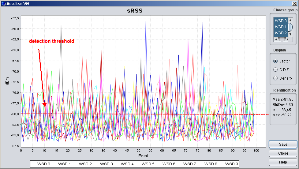
In such a scenario, the detection threshold is taken to a value of 0 dB (Figure 160) much higher than the sRSS level (average = -82.09 dBm) (Figure 161). Therefore, no victim system has been detected and the WSDs are allowed to transmit in any of the specified channels (Figure 162) per event.

Figure 160: Selection of a high detection threshold	Figure 161: The sRSS values are well below the detection threshold, so no victim system have been detected

 

In such a case the e.i.r.p.used in the simulation is the Tx_power (=-33 dBm) + G_max (=0 dBi), meaning that the in-block e.i.r.p. limit does not apply. This means that whatever the frequency selected by the WSD its e.i.r.p.. is the same (Figure 164) (here assuming that the Power Control at the It is OFF). 

Figure 162: The WSD can transmit anywhere in the victim frequency range	Figure 163: e.i.r.p. set to -33 dBm as set in the It, i.e. Txpower (=-33 dBm) + Gmax (=0 dBi), meaning that there were no limit applied to the It Tx power

 

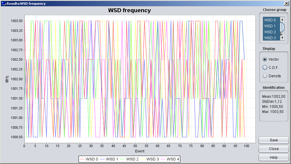
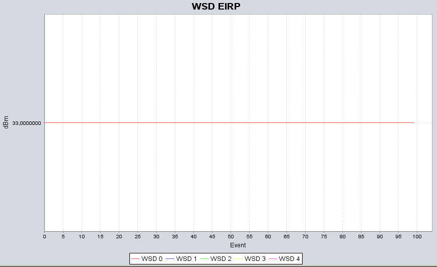
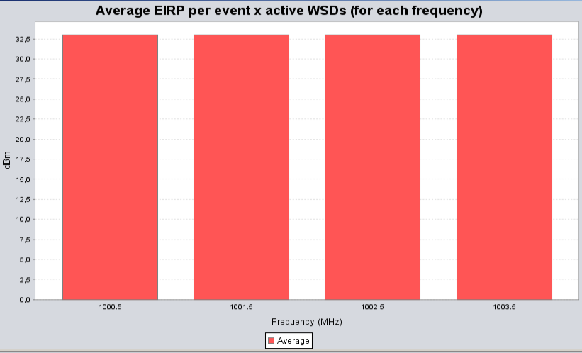
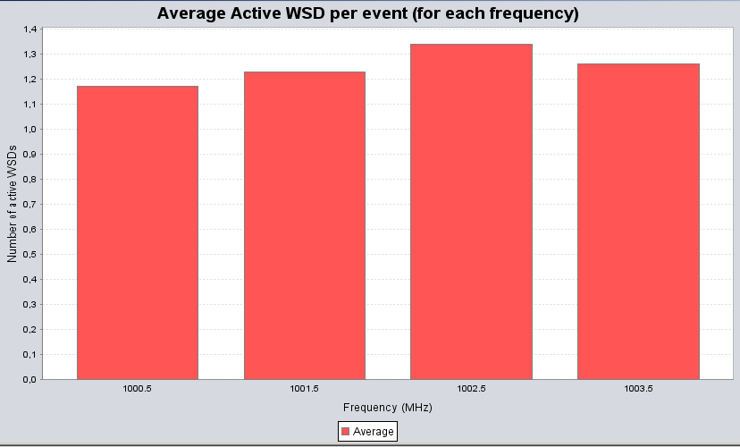
Figure 165 illustrates that on average there are 1.17 WSDs active at 1000.5 MHz per event, 1.23 WSDs in 1001.5 MHz, 1.34 WSDs in 1002.5 MHz and 1.26 WSDs in 1003.5 MHz for the same out of 5 which were input to the simulation. In this case all the WSDs were active (but in different frequencies) since the sum equal to 5 (i.e. none of the WSDs have been turned off).

Figure 164: e.i.r.p. is the same irrespective of the frequency	Figure 165: Illustration of the number of WSDs per frequency

6.5.2 All the channels are blocked

In such a scenario, the detection threshold is taken to a lower value compared to the sRSS and none of the WSDs are transmitting. In SEAMCAT, the Tx power is set to -1000 dBm (Figure 166). The WSD frequency is the same as the victim frequency per event. 

Figure 166: all the WSDs are off i.e. -1000 dBm

 

Note that in this specific case, the average e.i.r.p. and average WSDs per frequency can not be calculated and therefore can not be displayed as shown in Figure 168.

Figure 167: All the WSDs are off i.e. -1000 dBm

6.5.3 Some of the channels are blocked and some are available

This is a typical example. In such a scenario, the detection threshold is taken to a value of -80 dB (flat over the frequency range). This mean that when considering the sRSS of Figure 168, for some of the events, the sRSS will be above that threshold and therefore some WSDs will be considered as off (which explains the -1000 dBm value in Figure 169 (b)) and the WSD frequencies are randomly distributed.

(a) WSD frequency	(b) WSD e.i.r.p.

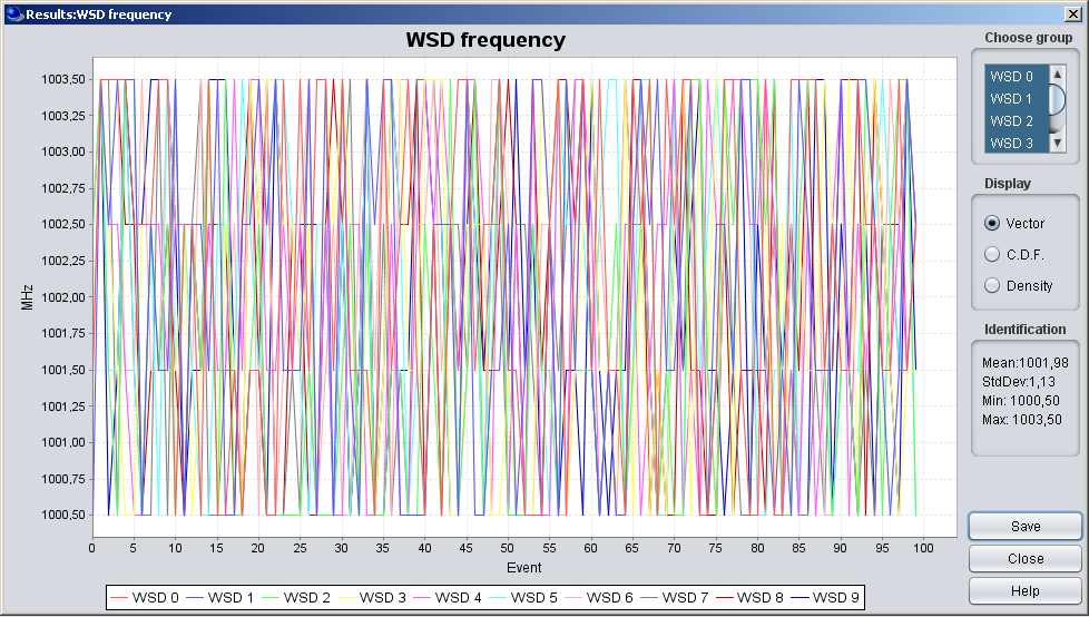
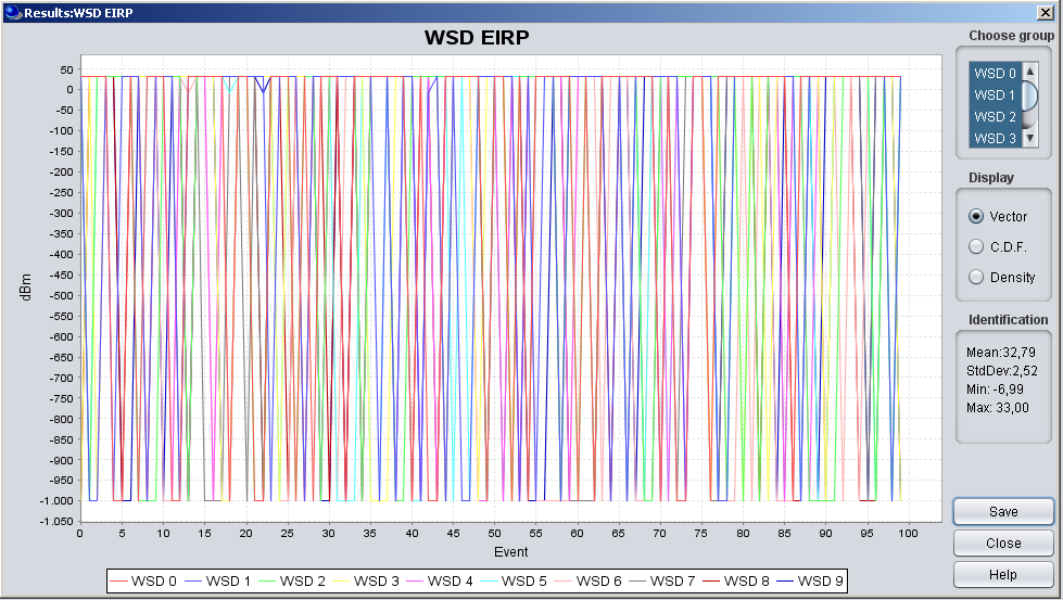
Figure 169: Output results of the WSD in (a) frequency and (b) e.i.r.p.

In this case, one can see that all the channels were occupied in Figure 170. The WSDs were allowed to transmit with an e.i.r.p. of 33 dBm in the 3 middle channels (1000.3 MHz to 1000.7 MHz) while for the side channels less power was allowed (i.e. 24 dBm for 1000.1 MHz and 16.89 dBm for 1000.9 MHz).

Figure 170 (b) also indicates that not all the simulated WSDs were active (those having an e.i.r.p. of -1000 dBm), and that per event about only 1 WSD was active.

 

(a) average e.i.r.p.	(b) average number of active WSDs

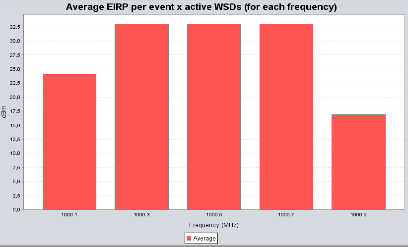
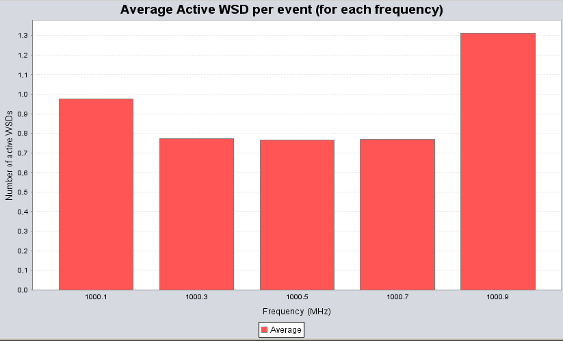
Figure 170: output results of the WSD in (a) frequency and (b) e.i.r.p.