5 Generic module

• 5.1 Generic system tab
• Intro
• 5.1.1 System
• 5.1.2 General
• 5.2 Receiver
• Introduction
• 5.2.1 Receiver identification
• 5.2.2 Antenna pointing
• 5.2.3 Antenna patterns identification
• 5.2.4 Reception characteristics
• 5.2.5 Interference criteria
• 5.3 Transmitter
• Introduction
• 5.3.1 Transmitter identification
• 5.3.2 Transmitter power
• 5.3.3 Transmitter antenna pointing
• 5.3.4 Antenna patterns identification
• 5.3.5 Emission characteristics
• 5.4 Transmitter to Receiver Path
• Introduction
• 5.4.1 Relative location
• 5.4.2 Coverage radius
• 5.4.3 Local environment
• 5.4.4 Propagation Model

5.1 Generic system tab

Intro

This tab allows you to update all scenario parameters of for a generic system .

In the upper part of the tab, you have three panels.

 

 

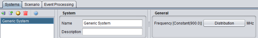
5.1.1 System

You can name and write some description of the victim system you want to simulate. 

5.1.2 General

The user can enter the frequency. The frequency value is overwritten at the “Scenario” tab level.

 

 You have access to 3 sub tabs to set the generic system:

• Receiver: This will be used either as VLR or ILR;

• Transmitter: This will beused either as VLT or ILT;

• Transmitter to Receiver Path (i.e. either VLT ->VLR or ILT ->ILR).

5.2 Receiver

Introduction

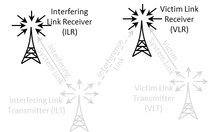
It can be the VLR or the ILR as illustrated in Figure 143.

 

 

The receiver consists of 5 panels (Figure 144); Receiver identification, antenna pointing, antenna patterns identification, reception characteristics and interference criteria.

 

 

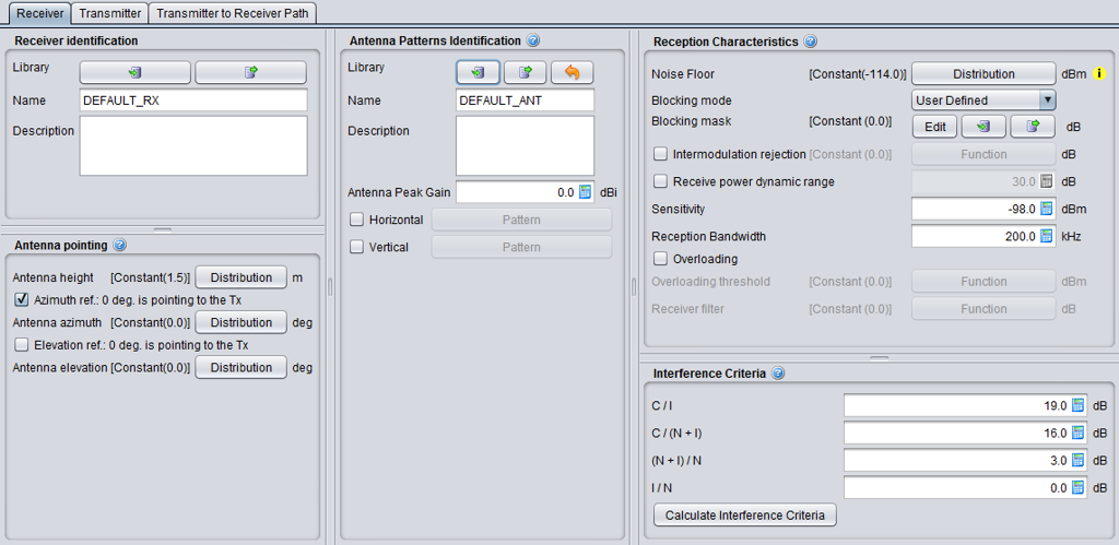
5.2.1 Receiver identification

This panel is a common interface that is reused in all other radio system.

 

 

5.2.2 Antenna pointing

This panel is a common interface that is reused in other radio system. It contains all information relative to the antenna other than the radiation pattern.

 

Table 10: Receiver antenna pointing GUI

5.2.3 Antenna patterns identification

This panel is a common interface that is reused in all other radio system. It contains all information relative to the antenna radiation pattern:

 

5.2.4 Reception characteristics

This panel consists in setting of the receiver characteristics of the generic system:

 

5.2.5 Interference criteria

Section 1.4 presented the concept of interference criteria (C/I, C/(N+I), (N+I)/N, I/N) when the victim is a generic system. The consistency between these values falls under the responsibility of the user. It should be noted that only one criterion is used at a time in the final interference calculation.

It is important to remember that these parameters are also used in the evaluation of the two blocking modes (Protection ratio and Sensitivity) as presented in See section 1.4.5.

SEAMCAT performs a consistency checking between the interference criteria as explained in ANNEX 3:.

 

The “calculate interference criteria” is a user friendly calculator for the interference criteria. It avoids conspicuous calculations, increases the transparency and avoids consistency check warnings because of the use of inconsistent sets of values.

The calculation and selection of a consistent set of interference criteria is implemented. The calculator opens with the existing values in the interference criteria fields of the workspace. A checkbox (default: ON) allows to force the consistency of the C/(N+I) value with the workspace, i.e. the values ‘Noise floor’ and ‘Sensitivity’. The relation between the values is given in the formula C/(N+I) [dB] = Sensitivity [dBm] – Noise floor [dBm]

The Interference Criteria Calculator displays all possible sets of consistent interference criteria rounded to two decimals. The same set is displayed only once. As a consequence of rounding, the displayed sets are differ at least 0.01 dB in one of the four values.

When you select the column of values you want and click ok, the values are copy/pasted to the “Interference criteria” panel.

 

 

 

5.3 Transmitter

Introduction

It can be the ILT or the VLT as illustrated in Figure 146.

 

 

It consists in 4 panels (Figure 147); Transmitter identification, antenna pointing, antenna patterns identification, emission characteristics. 

 

 

5.3.1 Transmitter identification

This is the same panel as in section 5.2.1 so that transmitter characteristics can be imported/exported from/to the library to/from the workspace and you can freely chose a name and a description.

5.3.2 Transmitter power

In SEAMCAT, the transmitter power (P) is expressed as conducted power in dBm, including feeder loss. The antenna peak gain (G) is expressed in dBi.

Consequently, the power calculated by SEAMCAT at the antenna output is the effective isotropic radiated power (e.i.r.p.) expressed in dBm:

e.i.r.p (dBm) = P (dBm)+G (dBi)

If the transmitter power is defined as e.i.r.p (dBm) or e.r.p (dBm), the conducted power (P), including feeder loss, can be calculated as follows:
P (dBm)= e.i.r.p (dBm)-G (dBi);
P (dBm)= e.r.p (dBm)-G (dBi)+2.15.

If the antenna gain is not known, it should be assumed zero, then:
P (dBm)= e.i.r.p (dBm);
P (dBm)= e.r.p (dBm)+2.15.
Note that G (dBi)= G (dBd)+2.15.

Example 1: P_t= 50 dBm (conducted transmitter power), L_f (feeder loss) = 2 dB, G_ant (antenna gain) = 15 dBi
SEAMCAT settings should be: Power (dBm) = 50 - 2 = 48, Antenna Peak Gain (dBi) = 15
e.i.r.p (dBm) calculated by SEAMCAT= P (dBm)+G (dBi) = 48 + 15 = 63 dBm

Example 2: e.i.r.p = 63 dBm, G_ant = 15 dBi, feeder loss in not needed
SEAMCAT settings should be: Power (dBm) = 63 - 15 = 48, Antenna Peak Gain (dBi) = 15
e.i.r.p (dBm) calculated by SEAMCAT= P (dBm)+G (dBi) = 48 + 15 = 63 dBm

Example 3: e.r.p = 60.85 dBm, G_ant = 12.85 dBd, feeder loss in not needed
SEAMCAT settings should be: Power (dBm)= 60.85 - 12.85 = 48, Antenna Peak Gain (dBi) = 12.85 + 2.15 = 15
e.i.r.p (dBm) calculated by SEAMCAT= P (dBm)+G (dBi) = 48 + 15 = 63 dBm

Example 4: e.i.r.p = 63 dBm, no other information available
SEAMCAT settings should be: Power (dBm) = 63, Antenna Peak Gain (dBi) = 0
e.i.r.p (dBm) calculated by SEAMCAT= P (dBm)+G (dBi) = 63 + 0 = 63 dBm

Example 5: e.r.p = 60.85 dBm, no other information available
SEAMCAT settings should be: Power (dBm) = 60.85, Antenna Peak Gain (dBi) = 2.15
e.i.r.p (dBm) calculated by SEAMCAT= P (dBm)+G (dBi) = 60.85 + 2.15 = 63 dBm

5.3.3 Transmitter antenna pointing

This is the same panel as in section 5.2.1 so that transmitter characteristics can be imported/exported from/to the library to/from the workspace and you can freely chose a name and a description.

5.3.4 Antenna patterns identification

It contains all information relative to the antenna radiation pattern. It is similar to the receiver antenna patterns identification (Section 5.2.3). 

5.3.5 Emission characteristics

This panel consists in setting of the emission characteristics of your generic system.

 

 

5.4 Transmitter to Receiver Path

Introduction

3 elements form the path between the VLR and the VLT or the ILR and ILT as illustrated in Figure 148.

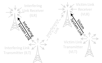
Figure 148: Transmitter to Receiver Path illustration

 

 

Figure 149: Transmitter to Receiver Path GUI

5.4.1 Relative location

• When the Correlated distance option is checked, the positions of the receiver and transmitter are geographically fixed with respect to each other (e.g. co-located or constantly spaced base stations). The transmitter is considered a reference centre.

• When the correlated distance is unchecked, the receiver is randomly moving around the transmitter. There are 2 primary options to define type of mutual placement of VLR with respect to VLT. 

See ANNEX 12: for further details on the algorithm and conventions. 

 

 

 

 

 

 

5.4.2 Coverage radius

A coverage radius is calculated for both the victim link and the interfering link. It is the

for the victim link (VLR-VLT) and the  for the interfering link (ILR-ILT) (see Annex A13.1). The receivers will be randomly deployed within the area centred on the transmitter and delimited by the coverage radius if the non-correlated option is selected.

 

Three different modes are available for calculating the maximum radius .

• User-defined radius allows directly entering the maximum radius (See Annex A13.1.1); 

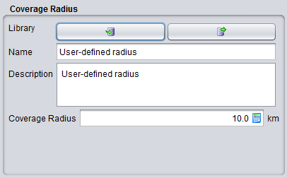
Figure 151: User-defined coverage radius dialog box

 

 

Table 16: Description on User-defined coverage radius

 

 

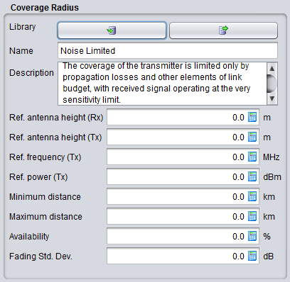
Figure 152: Noise limited network coverage radius dialog box

 

The coverage radius in the noise-limited network is defined by the parameters of Table 17. Note that the input parameters for the Noise-limited network interface are set to zero by default in order to independently define the radius from some parameters set elsewhere in the link.

 

 

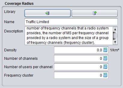
Traffic-limited network option will calculate the coverage radius, based on the formula for traffic-limited network. If this option is chosen, a set of input boxes will appear below allowing user to enter specific parameters required for this calculation (See Annex A13.1.3). 
    

 

The consistency of this parameter should be verified against the sensitivity, so that if a receiver is placed at given distance (e.g. at the maximum coverage radius) the received power is higher than the sensitivity for a reasonable percentage of occurrences (availability).

5.4.3 Local environment

The percentage of transceivers being indoor and outdoor can be selected thanks to this panel. It will work in combination with the chosen propagation model that you will select. By default the transmitter and receiver are located outdoor. For each elements of the link, it is possible to add   or remove   a probability of indoor.

 

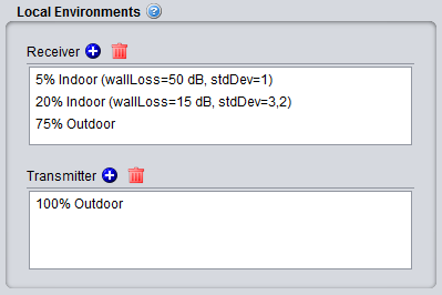Figure 154: Example of setting up the outdoor/indoor ratio

 

You can edit the field by double cliking

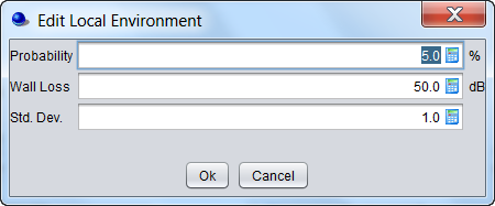Figure 155: Graphical interface to edit the probability, wall loss and associated standard deviation

 

 

Table 19: Local environment and wall loss

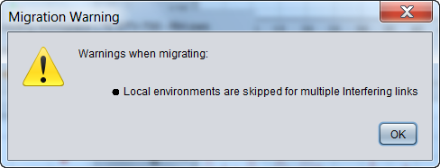
Note that when opening a workspace created prior to SEAMCAT version 5, all settings are mapped to the current SEAMCAT version running on your machine. As the parameter local environment didn’t exist before version 5, a warning may appear indicating that “local environments are skipped for multiple interfering links”. This means that SEAMCAT was not able to automatically set the parameters of the local environments (most likely due to a scenario with multiple interferers). Therefore, there is a need to edit the local environment manually.

 

5.4.4 Propagation Model

A suitable propagation model can be selected to be applied when calculating signal loss along the path between transmitters and receivers. Further information on propagation models are presented in detail in ANNEX 17.