# 4 Example of calculations
This section presents examples on how to use SEAMCAT to calculate Interference mechanism described in ANNEX 5:
# 4.1 iRSSunwanted
The following parameters should be changed in the simulation: (i) the interferer operates at 1000.3 MHz and (ii) outside the emission bandwidth, the attenuation is -23 dBc/200 kHz.
The corresponding power may derived using the known equation:
*(Eq. 20)*
[](https://wiki.cept.org/uploads/images/gallery/2026-04/LkF1IdJS3brKgBOD-image.png)
Then, in this example, outside the emission bandwidth (offset between –0.1 MHz and -1 MHz and between 0.1 MHz and 1 MHz), the power is equal to:
[](https://wiki.cept.org/uploads/images/gallery/2026-04/0yrjzOgCvrfjrVnp-image.png)
The complete unwanted emission mask is provided in the below figure.
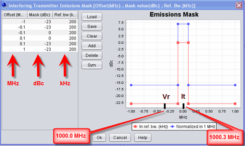
**Figure 99: Unwanted emission mask**
Using the previous assumptions, it is possible to derive the interfering power received by the Victim link receiver *within its bandwidth* as described in ANNEX 5: on page 274. This is called the iRSSunwanted:
*(Eq. 21)*
[](https://wiki.cept.org/uploads/images/gallery/2026-04/fjRmJOEE13LTjEVE-image.png)
[](https://wiki.cept.org/uploads/images/gallery/2026-04/qIi4YENJnbtoDGZm-image.png)
[](https://wiki.cept.org/uploads/images/gallery/2026-04/lDDTr6hKX9oaPRrP-image.png)
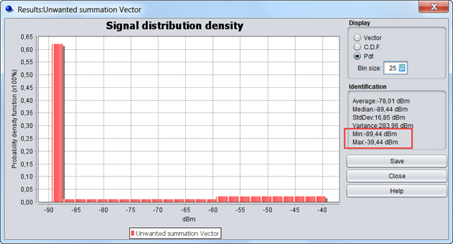
This can be checked by running a simulation and displaying the iRSSunwanted signal as depicted in Figure 100.
Figure 100: Mean iRSSunwanted

**In this example there is no bandwidth correction factor to be applied to the calculation of the iRSSunwanted since the VLR bandwidth and the ILT reference bandwidth have the same value (i.e. 200 KHz).**
**Examples of correction bandwidth can be found in section 3.3.8**
# 4.2 iRSSblocking
# Intro
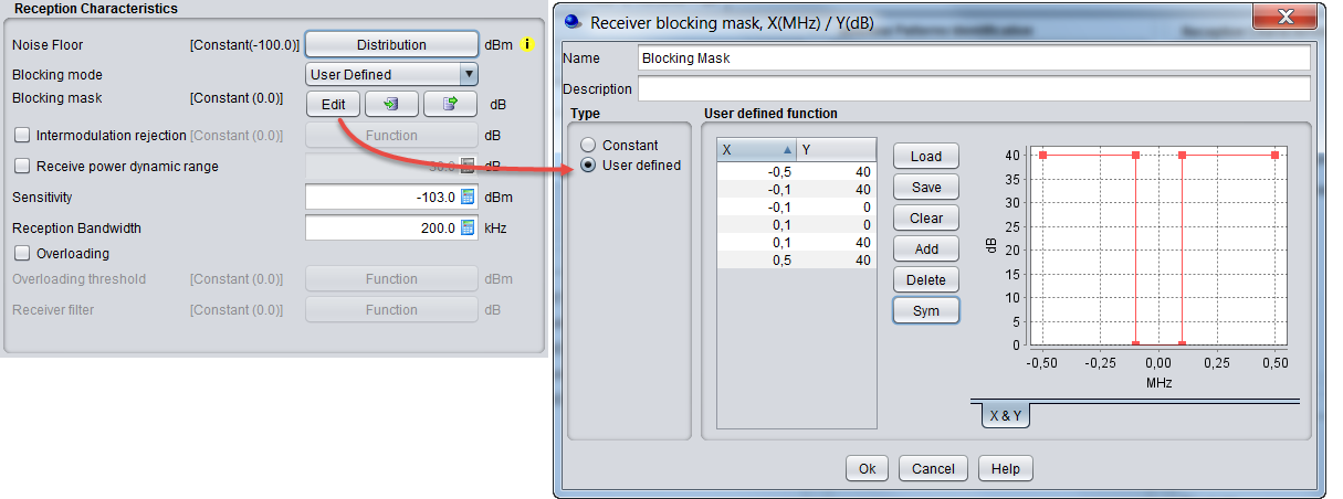
For this exercise, the blocking response from the receiver has a positive sign as shown in Figure 101. Detailed information on the calculation of the iRSSblocking can be found in section A5.2 of ANNEX 5:.
[](https://wiki.cept.org/uploads/images/gallery/2026-04/hvGEXeVhnLlYE5yE-image.png)
**Figure 101: Definition of the receiver blocking response**
# 4.2.1 User-defined mode
In this case, the Blocking is provided in dB and represents the attenuation of the receiver at a given frequency offset (see [A8.7](https://ecowiki.atlassian.net/wiki/spaces/SH/pages/492697 "https://ecowiki.atlassian.net/wiki/spaces/SH/pages/492697")). The resulting receiver attenuation equals the user-defined input values. Then, the iRSSblocking *at the interferer operating frequency * may be calculated as follows.
(***Note:** The ILT bandwidth is not considered in the iRSSblocking calculation*):
*(Eq. 22)*
[](https://wiki.cept.org/uploads/images/gallery/2026-04/EDEZPTaIeW2SuR77-image.png)
[](https://wiki.cept.org/uploads/images/gallery/2026-04/1riX8DbwQCEM50mx-image.png)
[](https://wiki.cept.org/uploads/images/gallery/2026-04/ihB6hCvvQNurn7ac-image.png)
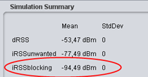
This can be checked by running a simulation and displaying the iRSSblocking in case of User-defined mode calculated by SEAMCAT. See the figure below.
# 4.2.2 Sensitivity mode
In this calculation mode the function *blockMax Interf Signal *(*Df*) that you entered represents the absolute power level (in dBm) of maximum interfering signal (maximum acceptable interfering power), which might be tolerated by the receiver at a given frequency separation (see [A8.7](https://ecowiki.atlassian.net/wiki/spaces/SH/pages/492697 "https://ecowiki.atlassian.net/wiki/spaces/SH/pages/492697")).
In this case SEAMCAT calculates the receiver attenuation, Attenuation (*Df*), to be applied to the interfering signal by using the following expression:
[](https://wiki.cept.org/uploads/images/gallery/2026-04/a4rFxolbIjEp2vdB-image.png)
where:
- D*f* = (*fILT - fVLR*) is the frequency separation;
- *sensVLR* is the sensitivity of the VLR (dBm) as defined in the simulation scenario.
To achieve a realistic value, you may define the sensitivity (*sensVLR*) as (see the figure below):
*Sensitivity = Noise Floor + C/(N+I)*
*Sensitivity = -110 dBm + 16 = -94 dBm*
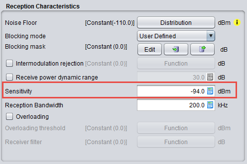
**Figure 103: Setting up the sensitivity in SEAMCAT**
Then the attenuation may be evaluated:
*Attenuation (Df ) = 40 + 94 + 16 - 0 = 150 dB*
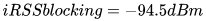
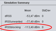
*iRSSblocking = Interfering Signal Level (f it )= -54.5 - 150 = -204.5 dBm*
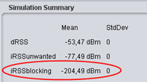
This can be checked by running a simulation and displaying the iRSSblocking in case of Sensitivity mode calculated by SEAMCAT see Figure 104.
# 4.2.3 Protection ratio
This mode is identical to the “sensitivity” mode since the only difference is that the Blocking value (relative to the noise floor) is provided in dB. The software processes the information using exactly the same method to obtain the value of the receiver attenuation (see [A8.7](https://ecowiki.atlassian.net/wiki/spaces/SH/pages/492697 "https://ecowiki.atlassian.net/wiki/spaces/SH/pages/492697")).
The function *blockProtection Ratio*(*Df*) that you entered represents the protection ratio, i.e. the ratio of maximum acceptable level of interfering signal to the wanted signal level, at a given frequency separation.
In this case SEAMCAT calculates the receiver attenuation *aVLR*(*Df*) to be applied to the interfering signal by using the following expression (see Figure 105):
*(Eq. 24)*
[](https://wiki.cept.org/uploads/images/gallery/2026-04/GZW81QnpOQGHceTW-image.png)
[](https://wiki.cept.org/uploads/images/gallery/2026-04/7bMtDiIykGnBdjjZ-image.png)
[](https://wiki.cept.org/uploads/images/gallery/2026-04/xR43Rds7Q0tzHqSr-image.png)
[](https://wiki.cept.org/uploads/images/gallery/2026-04/n8ZFCYfy45LY4C7J-image.png)
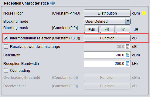
# 4.3 iRSSintermodulation
The following graphics presents the input parameters to activate when the intermodulation mechanism is to be investigated. The intermodulation rejection mask is expressed in dB versus frequency offset (MHz). Results details can be found in Section 12.3.3.
[](https://wiki.cept.org/uploads/images/gallery/2026-04/mODaXVPPBqxelfKf-image.png)
# 4.4 iRSSoverlaoding
The following graphics presents the input parameters to activate when the overloading mechanism is to be simulated.
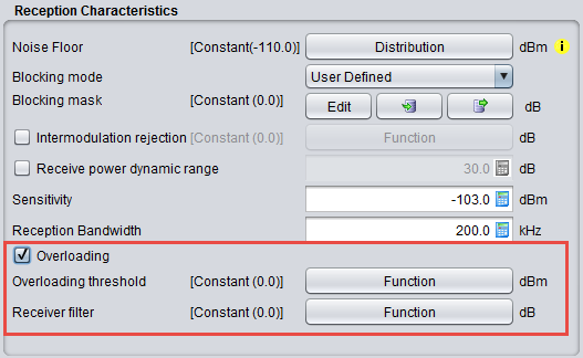
The overloading mask is expressed in power (dBm) versus frequency offset (MHz) and is defined as a function in SEAMCAT.
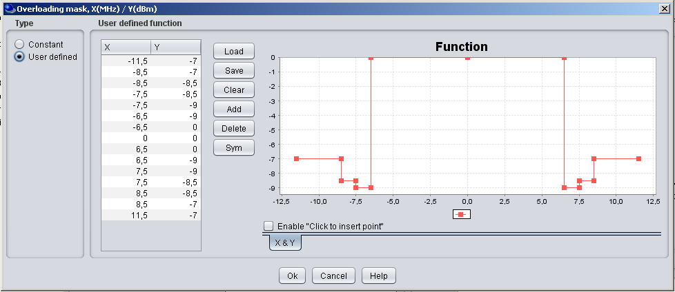
**Figure 108: Setting of the overloading mask in SEAMCAT**
The filtering of the receiver is expressed in power (dB) versus frequency offset (MHz) and is defined as a function in SEAMCAT (see Figure 109). It is set by default to a constant value of zero.
Note that if the blocking attenuation mode in user-defined and the overloading feature have been selected, then a consistency check will remind you that the actual blocking response and the receiver filter are the same element and they should not be accounted twice.
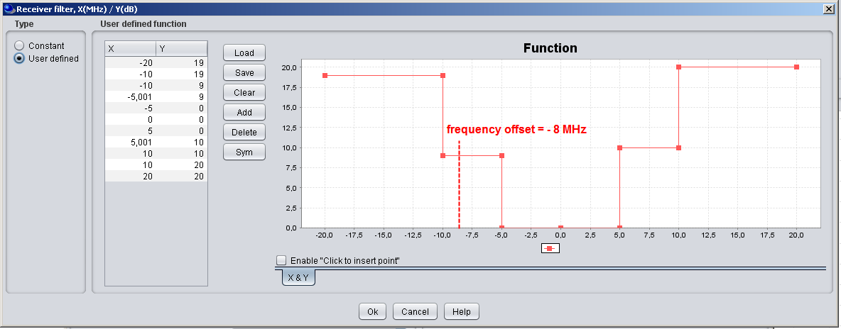
**Figure 109: Example of filling the Rx filter function**
When a simulation is run the following results are extractable (see Section 12.3.4 for further details)
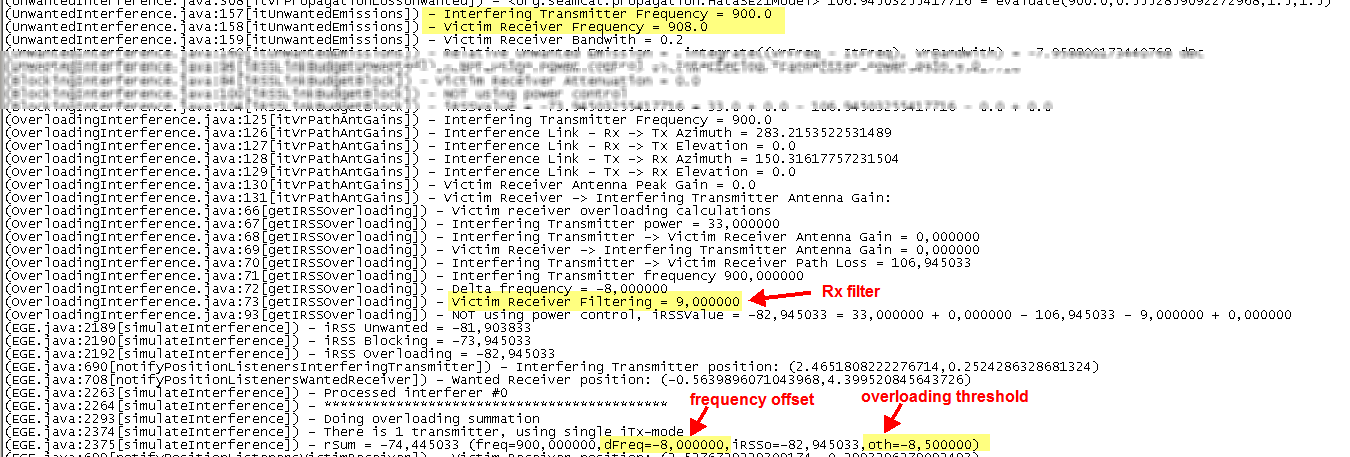
As an example, this means that for the following overloading mask presented in Figure 3 with a victim frequency of 908 MHz and an interfering frequency of 900 MHz, the delta frequency (i.e. frequency offset) is -8 MHz with an overloading treshold of -8.5 dB and a Rx filter value of 9 dB. This can be found from the log file as shown below in Figure 110.
[](https://wiki.cept.org/uploads/images/gallery/2026-04/HSGBixvqvMZCbAPP-image.png)
[](https://wiki.cept.org/uploads/images/gallery/2026-04/IfSqb4xgaawTpjTX-image.png)
# 4.5 Coverage radius (VLR-VLT)
In this section the Free Space Model is used to derive the attenuation on the different paths and the Victim Link and Interfering Link operate at the same frequency – 1000 MHz – co-channel interference. Figure 115 presents an illustration of the various radii (i.e. coverage radius and simulation radius) that are used in SEAMCAT and with reference to the various pairs of transmitters and receivers used for a simulation.
[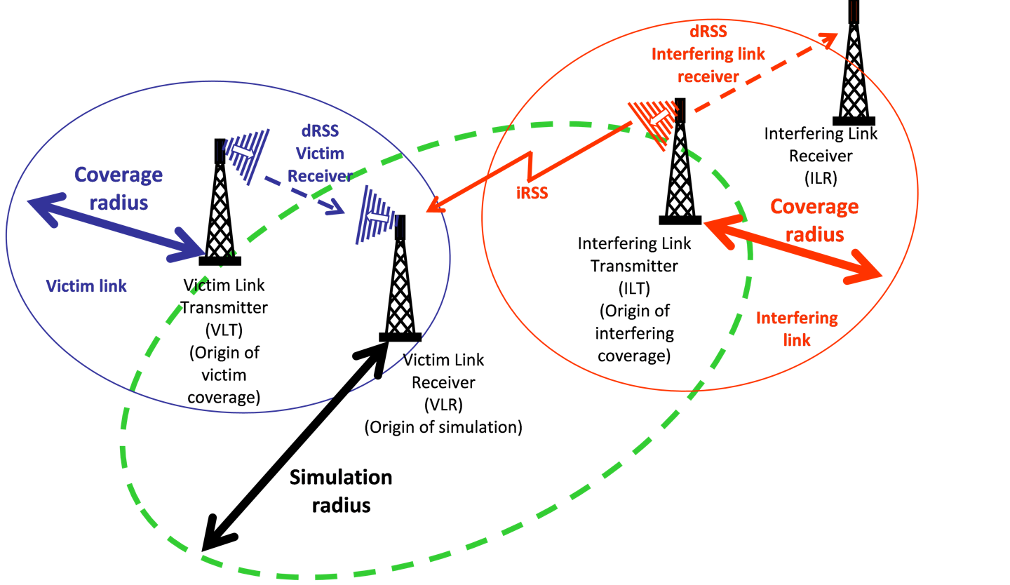](https://wiki.cept.org/uploads/images/gallery/2026-04/U4WR81sjGYmWlWjD-image.png)
**Figure 111: Illustration of the Coverage Radius and the Simulation Radius with respect to the pairs of transmitters and receivers of the victim and interfering links**
The distance between the VLT and the VLR is referred to as the **coverage radius (**[](https://wiki.cept.org/uploads/images/gallery/2026-04/lbSA5AJdIlxVYd5i-image.png)**)** (see ANNEX 13:**)**. In the case of mobile applications, the number of terminals that may transmit in a given cell of the network is given by:
[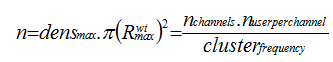](https://wiki.cept.org/uploads/images/gallery/2026-04/sbD1eUt2rCB9fjE9-image.png)
**Figure 112: Frequency cluster**
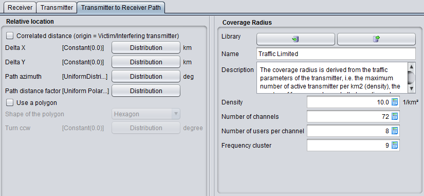
The victim link coverage radius (i.e. centred on the victim link transmitter) may then be calculated by using the formula below. Figure 113 presents how to set-up SEAMCAT.
[](https://wiki.cept.org/uploads/images/gallery/2026-04/DJuUlRiUNO9WpjLf-image.png)
(Eq. 26)
[](https://wiki.cept.org/uploads/images/gallery/2026-04/p0QT5Yzfr0ELqceG-image.png)
(Eq. 27)
[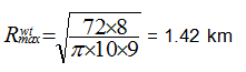](https://wiki.cept.org/uploads/images/gallery/2026-04/fhCijQoGISQpTgM7-image.png)
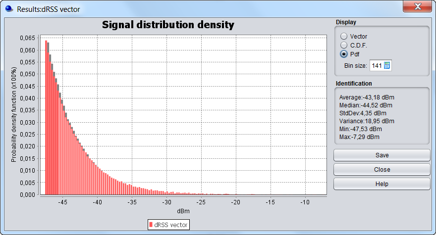
Figure 115 presents the results of the dRSS vector and the results in the coverage radius of the victim link.
The dRSS for a receiver located at the edge of the coverage area may be calculated:
*dRSS = 30 (dBm) + 9 + 9 - (32.5 + 10 log(1.43^2) + 20 log(1000)) = -47.5 dBm*
[](https://wiki.cept.org/uploads/images/gallery/2026-04/vS1j6ax2beFdaJzk-image.png)
[](https://wiki.cept.org/uploads/images/gallery/2026-04/DpFF0zTI0YyX535k-image.png)
[](https://wiki.cept.org/uploads/images/gallery/2026-04/WpalcPn1uaLqprJi-image.png)
# 4.6 Simulation radius (ILT-VLR)
The distance between the Victim link receiver and the Interfering link transmitter is referred to as the **simulation radius** (see ANNEX 13:**)**. It can be defined as shown in Figure 117.
[](https://wiki.cept.org/uploads/images/gallery/2026-04/AXHxWiUXVnRPafzK-image.png)
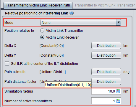
Using this feature, the interfering link transmitter is located between 1 km (0.1 x 10 km) and 10 km (1 x 10 km) from the Victim link receiver as shown in the SEAMCAT display in Figure 118.
[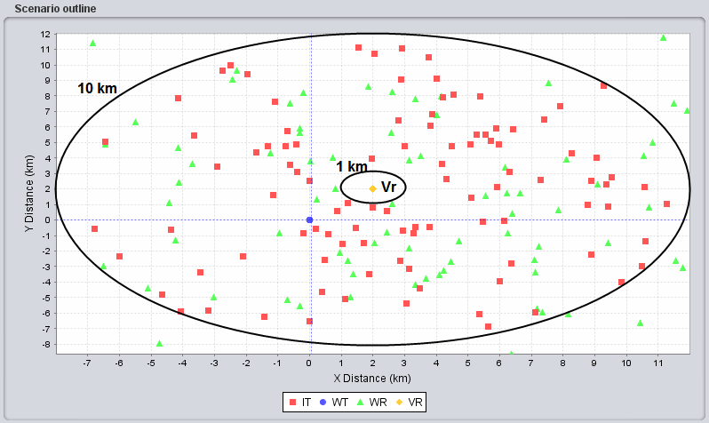](https://wiki.cept.org/uploads/images/gallery/2026-04/PJnf8gxRGbfbLRio-image.png)**Figure 118: SEAMCAT display of the minimum distance**
(ILT-red, ILR-green, VLR-yellow, VLT-blue)
If the interefering link transmitter is located at 10 km, it is possible to derive the iRSSunwanted:
[](https://wiki.cept.org/uploads/images/gallery/2026-04/2b9EHgA9tp6b4UcX-image.png)
[](https://wiki.cept.org/uploads/images/gallery/2026-04/ZL3CIi7kJXbTBGeY-image.png)
If the interefering link transmitter is located at 1 km:
[](https://wiki.cept.org/uploads/images/gallery/2026-04/6MsuO8ypcS4wqPTU-image.png)
[](https://wiki.cept.org/uploads/images/gallery/2026-04/raQtskKNclLPCOjJ-image.png)
The iRSSunwanted extends from -59.5 dBm to -39.5 dBm as confirmed by Figure 119.
[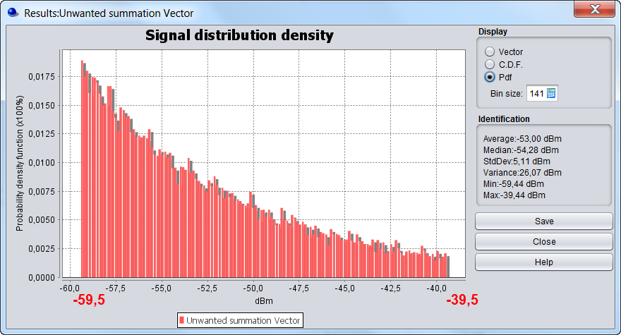](https://wiki.cept.org/uploads/images/gallery/2026-04/UOB88eJnGy75zK7F-image.png)
# 4.7 Uniform distribution of ILT vs VLR
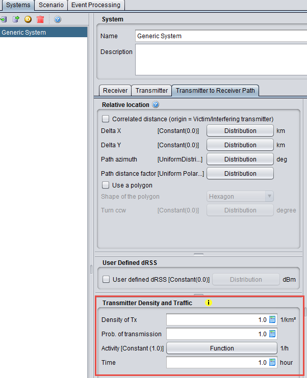
You may define a uniform deployment density of terminals/transmitters per km (see ANNEX 13:**).** This can either be done by using the “**Uniform Density” mode** combined with the calculation of a simulation radius as described in section 4.7.1 and A13.2 or by using the “**none” mode** combined with the choice of uniform path polar distance as described in section 4.7.2.
# 4.7.1 Uniform density mode - simulation radius calculation
[](https://wiki.cept.org/uploads/images/gallery/2026-04/YL3nDQffwX4mxQjq-image.png)
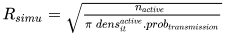
The number of active transmitters that will be uniformly located within the simulation radius is given by:
[](https://wiki.cept.org/uploads/images/gallery/2026-04/fxk5lJJMVsi3fXBU-image.png) (Eq. 28)
Figure 120 presents the GUI with the input value.
| **Settings in the System tab** | **Settings in the Scenario tab** |
| [](https://wiki.cept.org/uploads/images/gallery/2026-04/QQsGwc78HTIcPgZs-image.png)
| [](https://wiki.cept.org/uploads/images/gallery/2026-04/hK5xBs1NucCNErqS-image.png)
|
**Figure 120: Setting up the simulation radius in SEAMCAT** (Note that the results of the simulation radius is displayed only after running simulation)
The simulation radius is calculated by using the following formula:
[](https://wiki.cept.org/uploads/images/gallery/2026-04/QzbhPAAHF1adgLWw-image.png) (Eq. 29)
In the example of Figure 120, this gives:
[](https://wiki.cept.org/uploads/images/gallery/2026-04/vTJB5YDQbnyRfe5h-image.png)
[](https://wiki.cept.org/uploads/images/gallery/2026-04/J00mjnYWTj1GFptH-image.png)
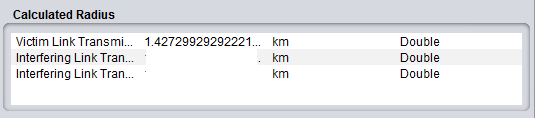
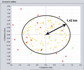
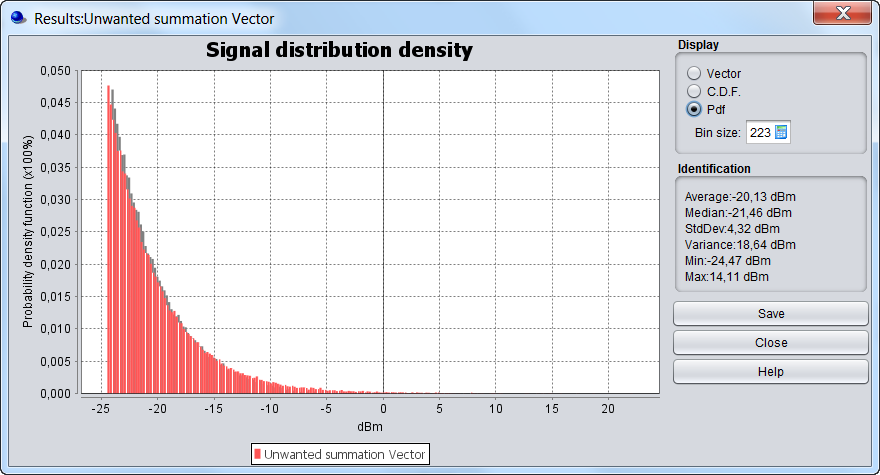
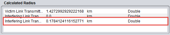
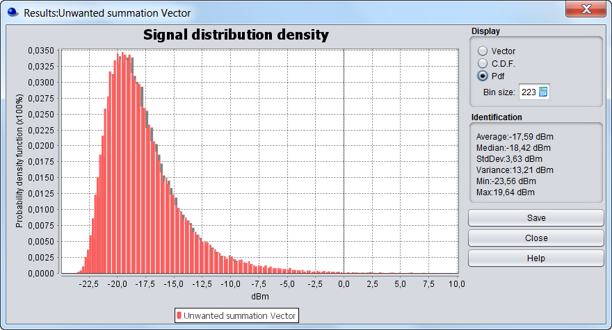
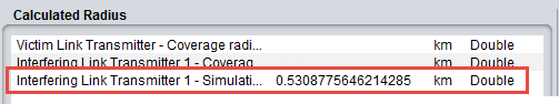
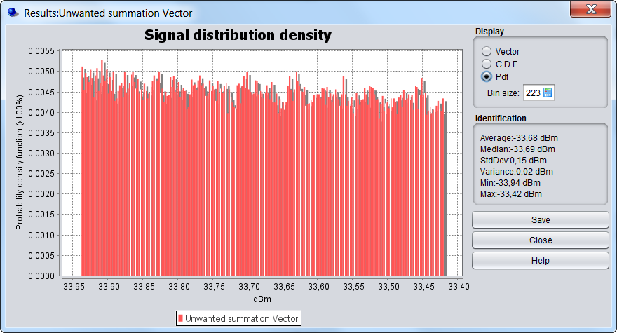
Then for a ***single*** interefering link transmitter located at the edge of the simulation radius (R = 0.178 km), the iRSSunwanted may be calculated:

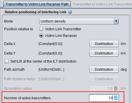
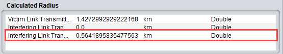
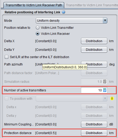
When increasing the number of active transmitters to 10 (see Figure 123), the simulation radius becomes:
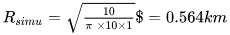
Then, for a ***single*** interefering link transmitter located at the edge of that simulation radius (R = 0.564 km), the iRSSunwanted resulting from this terminal may be calculated as:

If 10 active terminals are located at the edge of the simulation radius, the iRSSunwanted may be calculated in the following way:

[](https://wiki.cept.org/uploads/images/gallery/2026-04/nvWwpk7aBs0QgxNH-image.png)**Figure 125: Calculated simulation radius with 10 active transmitters**
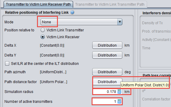
# 4.7.2 "None" mode
When you select the “**None” mode** (see ANNEX 13:**)**, he can also define a Uniform density of terminal/transmitter by using the Uniform polar distance defined within the path distance factor and a uniform distributed path azimuth (0 to 360 deg).**Uniform polar distance** leads to uniformly distributed terminals in the **circular area** (area) and the **Uniform distance** leads to uniformly distributed terminals along the **radius** (line).
Then using a user-defined radius of 0.178 km and 1 interefering link transmitter (see Figure 126), it is possible to reproduce the results of section 4.7.1. Therefore, the same results as those given in Figure 121 are found as shown in Figure 127.
[](https://wiki.cept.org/uploads/images/gallery/2026-04/FgDVJXDdtN0Axq5W-image.png)
[](https://wiki.cept.org/uploads/images/gallery/2026-04/fGqs2Po67vV5PHG3-image.png)**Figure 127: iRSSunwanted / Uniform polar feature / 1 interfering link transmitter and simulation radius of 0.178 km (same results as in Figure 121)**
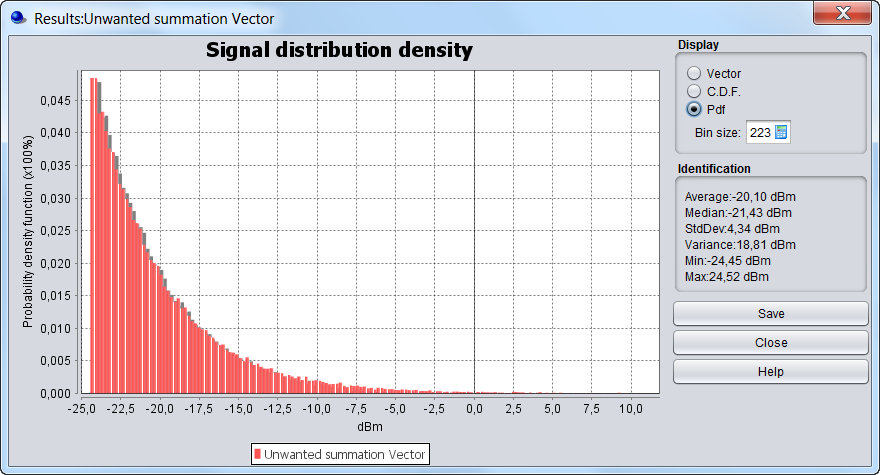
Using a user-defined radius of 0.564 km and 10 interefering link transmitters, the same results as those given in Figure 124 are reached as shown in Figure 128.
[](https://wiki.cept.org/uploads/images/gallery/2026-04/K2MeRcMFiI8jwZkK-image.png)
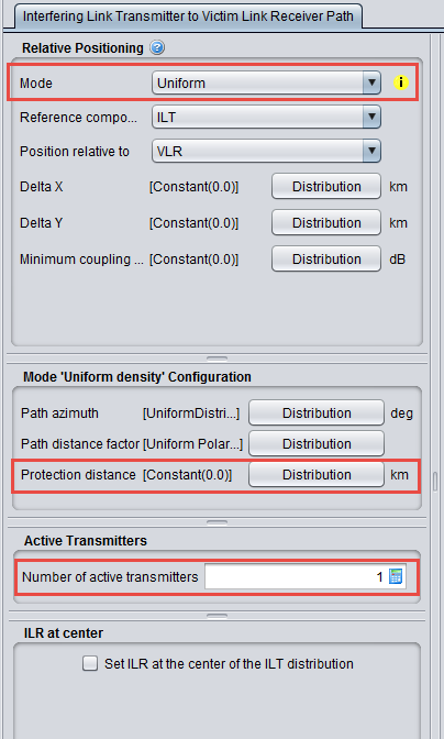
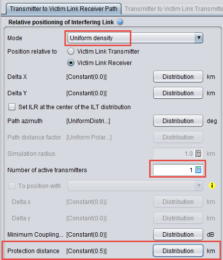
# 4.8 Protection distance
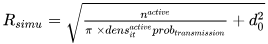
If a minimum protection distance between the victim link receiver and interfering link transmitter is introduced then the simulation radius may then be calculated by using the following formula:
[](https://wiki.cept.org/uploads/images/gallery/2026-04/pwgpa7jGvwzhp4Id-image.png) *(Eq. 30)*
Note: The calculation of the iRSS at each trial will be performed only if the location of the ILT satisfies the following condition[](https://wiki.cept.org/uploads/images/gallery/2026-04/TjRdjTaR2Noryw4a-image.png).
Figure 129 presents how to set-up SEAMCAT (See also A13.2 for further details).
[](https://wiki.cept.org/uploads/images/gallery/2026-04/I56kzfMBz4PrxcYi-image.png)
The simulation radius (see Figure 131) may then be calculated by using the following formula:
[](https://wiki.cept.org/uploads/images/gallery/2026-04/TB0VHNJzFkdblD1q-image.png)
[](https://wiki.cept.org/uploads/images/gallery/2026-04/wejZFOOKud5ggpOl-image.png)
**Figure 130: Calculated simulated radius**
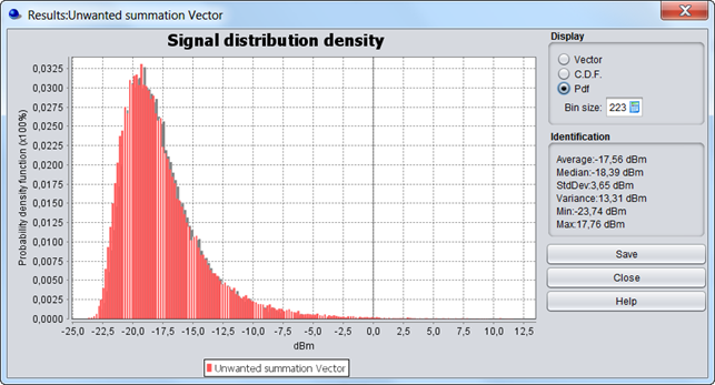
If the distance between the VLR and the ILT is equal to the protection distance (0.5 km), then:
[](https://wiki.cept.org/uploads/images/gallery/2026-04/7kNdDJc7jZjPjPsF-image.png)
If the distance between the VLR and the ILT is equal to the simulation radius (0.531 km), then:
[](https://wiki.cept.org/uploads/images/gallery/2026-04/bKY9chLl8plNC8bT-image.png)
These results are in line with those depicted on Figure 131. We can then increase the number of active transmitters to 10 as shown in Figure 132.
[](https://wiki.cept.org/uploads/images/gallery/2026-04/Q5mewLud0E5vG5Hv-image.png)
The simulation radius may then be calculated by using the following formula (see Figure 133 for the result):
[](https://wiki.cept.org/uploads/images/gallery/2026-04/pv3sdy5GazLQO9wg-image.png)
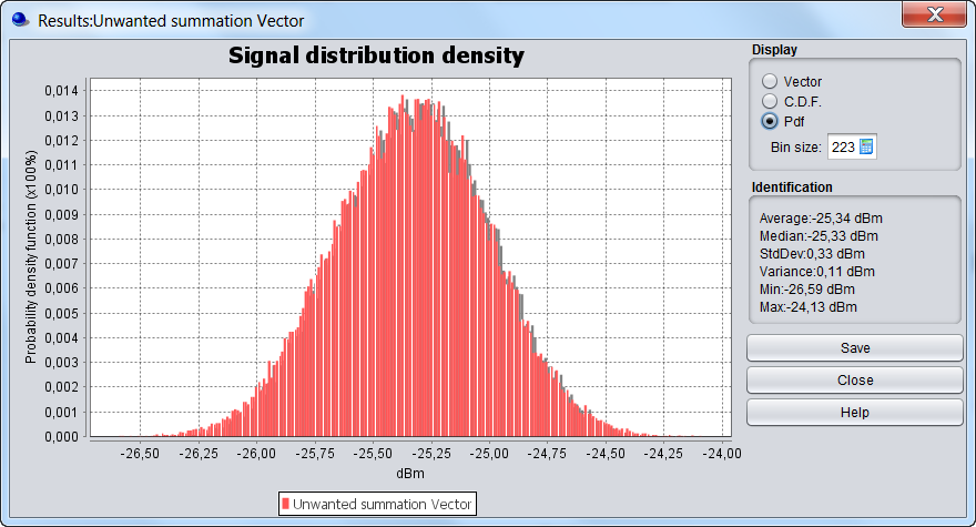**Figure 133: Calculation of the Rsimu and the iRSSunwanted using the protection distance**
**(*****for 10 active interferer*****)**
If the distance between the VLR and a single ILT is equal to the protection distance, then:
[](https://wiki.cept.org/uploads/images/gallery/2026-04/pOpLzDjuY2wdeRRo-image.png)
If the distance between the VLR and a single ILT is equal to the simulation radius, then:
[](https://wiki.cept.org/uploads/images/gallery/2026-04/mQKnfQhcrwMrs2QP-image.png)
If 10 transmitters are deployed around the VLR then:
[](https://wiki.cept.org/uploads/images/gallery/2026-04/GBABDSpjusnHin5B-image.png) and
[](https://wiki.cept.org/uploads/images/gallery/2026-04/a0upNbBP9IkyLQ7z-image.png)
[](https://wiki.cept.org/uploads/images/gallery/2026-04/ACjfhTVThiN8Oyqu-image.png) *(see Figure 133)*
# 4.9 Power Control
**Note:** The power control is used only in this section. When considering other sections, the power control feature should be deactivated.
A power control feature is implemented within SEAMCAT. When this feature is activated it introduces a variation of the interefering link transmitter power. More details on the implementation of the power control in SEAMCAT is presented in ANNEX 14:.
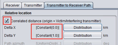
When using the scenario provided in section 3 (Victim Link and Interfering Link operate at the same frequency 1000 MHz but with a interfering link receiver antenna gain should be equal to 11 dBi), it becomes possible to define the distance between the Victim link receiver and the Interefering link transmitter.
For simplification, we consider that the Victim link receiver and the Interefering link transmitter are defined using the following assumptions (1 km distance between the Victim and the Interefering link transmitter). This is illustrated in Figure 134.
[](https://wiki.cept.org/uploads/images/gallery/2026-04/3eM4rgLenmG8JvB8-image.png)
If the power control is not activated then the iRSSunwanted is (see Figure 135):
[](https://wiki.cept.org/uploads/images/gallery/2026-04/DPI21oN67HJzB8Di-image.png)
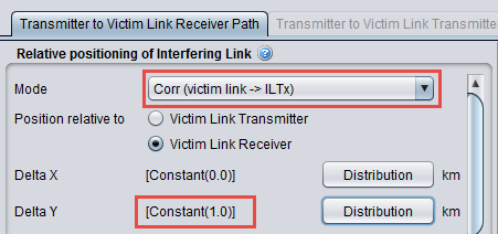
The same assumption is used for the distance between ILT and the ILR (i.e. x = 0 km and y = 1 km) where the ILT is the (0,0) origin as shown in Figure 136.
The power received by the Interfering link receiver (dRSSInterfering link receiver) is then:
[](https://wiki.cept.org/uploads/images/gallery/2026-04/rkltmy8znVTkHQsc-image.png)
Note: ***You should not confuse the dRSSInterfering link receiver and the dRSSVictim link receiver. Figure 111 illustrates their differences.***
The power control can be input as shown in Figure 137.
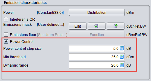
Using these assumptions, the results of the simulation are the same as previously since the threshold (-35 dBm) is above the dRSSInterfering link receiver (-37.5 dB). This corresponds to the Case 1 described in ANNEX 14:.
Now, if the threshold is decreased from –35 dBm to –50 dBm (see Figure 138)
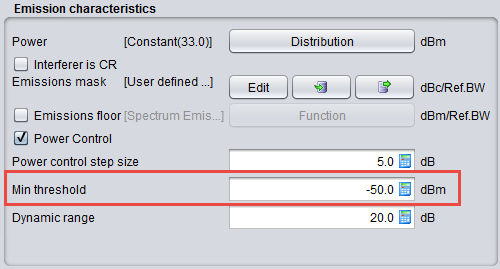
Since, the power control feature is activated the gain of the power control is determined according to the guidance given in ANNEX 14: on page 344. Since the dRSSInterfering link receiver is –37.5 dBm and:

The gain of the power control (*git PC*) is 10 dB (Case (i+1) in ANNEX 14:). This means that the iRSSunwanted will be decreased by 10 dB, i.e. :

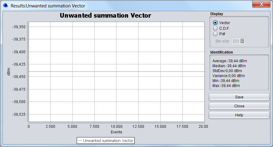
Finally, if the threshold is decreased from –50 dBm to –70 dBm, the power control feature is activated. Since the dRSSInterfering link receiver is –37.5 dBm, this results in:

The gain of the power control is 20 dB (Case (*n\_step* + 2) in ANNEX 14:). This means that the iRSSunwanted will be decreased by 20 dB, i.e. :
[](https://wiki.cept.org/uploads/images/gallery/2026-04/VjjtboR6gjSqrE32-image.png)
# 4.10 Antenna gain
For simplification, we consider that the Victim link receiver and the Interfering link transmitter are defined using the following assumptions (again 1 km distance between the Interfering link transmitter and the Victim link receiver).
The iRSSunwanted is then:
*iRSSunwanted = 33 (dBm) + 11 + Gr - (32.5 + 10 log(1) + 20 log(1000)) = -48.5 dBm + Gr*
[](https://wiki.cept.org/uploads/images/gallery/2026-04/nVmKNumNAo7c2juY-image.png)
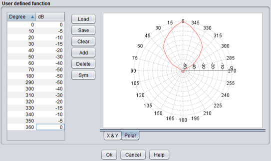
In order to investigate the evolution of the iRSS versus the antenna radiation pattern with fixed location of the pairs of transmitters and receivers (i.e. to get random angle arrival and consequently random gain of the antenna radiation pattern), it is possible to rotate artificially the antenna pattern defined in Figure 139 in the azimuth domain. This can be done by rotating the antenna from 0 to 360 by applying a uniform distribution from 0 to 360 deg to the main beam direction (0 deg).
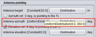
**Figure 140: Setting up the rotation in the azimuth domain**
The receiver antenna gain extends from 9 dB + (0 to -50 dB) meaning that it varies from +9 dB to -41 dB depending on the azimuth angle (Figure 140), the iRSSunwanted is then :
*-89.5 dBm < iRSSunwanted < -39.5 dBm*
Results generated by SEAMCAT are presented in Figure 141.