4.7 Uniform distribution of ILT vs VLR
You may define a uniform deployment density of terminals/transmitters per km (see ANNEX 13:). This can either be done by using the “Uniform Density” mode combined with the calculation of a simulation radius as described in section 4.7.1 and A13.2 or by using the “none” mode combined with the choice of uniform path polar distance as described in section 4.7.2.
4.7.1 Uniform density mode - simulation radius calculation

The number of active transmitters that will be uniformly located within the simulation radius is given by:
 (Eq. 28)
Figure 120 presents the GUI with the input value.
| Settings in the System tab | Settings in the Scenario tab |
|
|
|
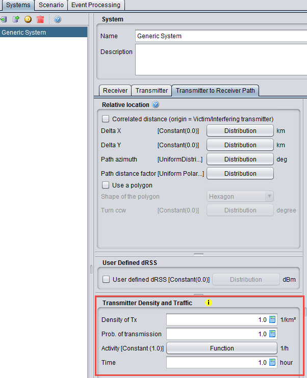

Figure 120: Setting up the simulation radius in SEAMCAT
(Note that the results of the simulation radius is displayed only after running simulation)
The simulation radius is calculated by using the following formula:
 (Eq. 29)
In the example of Figure 120, this gives:


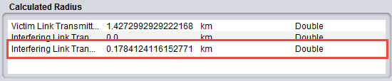
Then for a single interefering link transmitter located at the edge of the simulation radius (R = 0.178 km), the iRSSunwanted may be calculated:

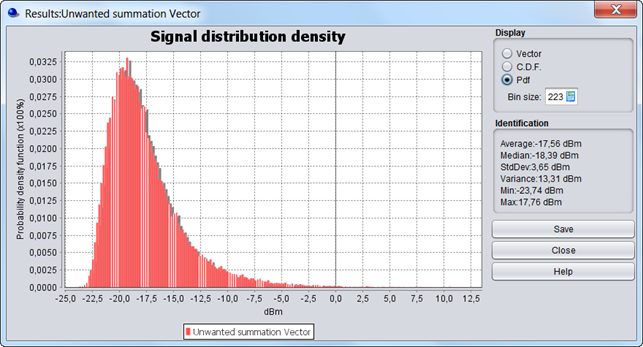
When increasing the number of active transmitters to 10 (see Figure 123), the simulation radius becomes:

Then, for a single interefering link transmitter located at the edge of that simulation radius (R = 0.564 km), the iRSSunwanted resulting from this terminal may be calculated as:

If 10 active terminals are located at the edge of the simulation radius, the iRSSunwanted may be calculated in the following way:


number of active transmitters

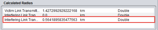 Figure 125: Calculated simulation radius with 10 active transmitters
4.7.2 "None" mode
When you select the “None” mode (see ANNEX 13:), he can also define a Uniform density of terminal/transmitter by using the Uniform polar distance defined within the path distance factor and a uniform distributed path azimuth (0 to 360 deg).Uniform polar distance leads to uniformly distributed terminals in the circular area (area) and the Uniform distance leads to uniformly distributed terminals along the radius (line).
Then using a user-defined radius of 0.178 km and 1 interefering link transmitter (see Figure 126), it is possible to reproduce the results of section 4.7.1. Therefore, the same results as those given in Figure 121 are found as shown in Figure 127.
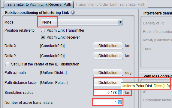
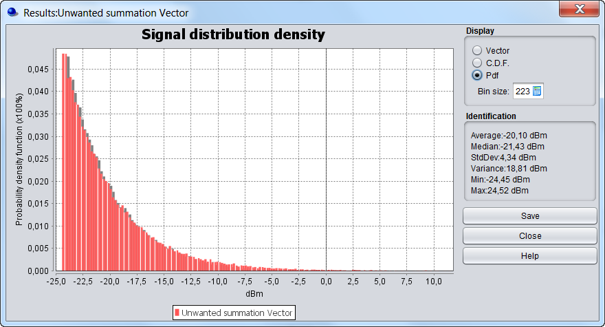 Figure 127: iRSSunwanted / Uniform polar feature / 1 interfering link transmitter and simulation radius of 0.178 km (same results as in Figure 121)
Using a user-defined radius of 0.564 km and 10 interefering link transmitters, the same results as those given in Figure 124 are reached as shown in Figure 128.
(same results as in Figure 121)