3 Example of running a simulation

• 3.1 Setting the scenario
• 3.2 Calculating the dRSS
• 3.2.1 Victim link
• 3.2.2 System to be a victim
• 3.2.4 Transmitter
• 3.2.5 Positioning the VLT vs VLR
• 3.2.6 Selecting the propagation model
• 3.2.7 Calculating the dRSS by hand
• 3.2.8 Export/import your system to library
• 3.2.9 Selecting the victim in the Scenario
• 3.3 Calculating the iRSS
• 3.3.0 Objective
• 3.3.1 Interfering Links
• 3.3.2 System to be an interferer
• 3.3.3 Transmitter
• 3.3.4 Receiver
• 3.3.5 Positioning of the ILT vs ILR
• 3.3.6 Positioning of the VLR vs ILT
• 3.3.7 Calculating the iRSS by hand
• 3.3.8 Emission, reference, VLR bandwidth relationship and bandwidth correction factor
• 3.4 Launching a simulation
• 3.5 Extract results vectors (dRSS, iRSS etc...)
• 3.6 Calculating the probability of interference
• Objective
• 3.6.1 Compatibility calculation mode
• 3.6.2 Translation calculation mode
• 3.6.3 Example of probability of interference calculation

3.1 Setting the scenario

 

Running a simulation consists essentially in setting the input parameters of the victim and the interfering system according to your requirement. Similarly, you need to consider the requirement of the geographical location of the various systems. For this example, let’s consider a fixed link, which is interfered by another fixed link as illustrated in Figure 64.

The Victim link transmitter and the Victim link receiver compose the “Victim link” and the Interefering link transmitter and the Interfering link receiver compose the “Interfering Link”.

Figure 64: Example of Application of SEAMCAT

3.2 Calculating the dRSS

3.2.1 Victim link

The victim parameter characteristics summarised in Table 6 should be entered into SEAMCAT.

 

 Each simulation workspace contains one and only one victim link. 

3.2.2 System to be a victim

In order to set up a workspace, the first step is to set the system that will be used as victim: set the characteristics of the receiver  (that will be the victim link receiver (VLR)) and the transmitter (that will be the victim link transmitter (VLT)).

System characteristics can be directly edited in the system tab. This is illustrated in the figure below.

 

Figure 65: Access to the system environment

For example, a generic system can be selected from the “import system from library button” as shown Figure 67.

 

Figure 66: Import system from library button

 

Figure 67: Selecting a system from library

 

 

First, let set the frequency of the victim. The frequency can be changed from 900 MHz (default value) to 1000 MHz as described in Figure 68. In this example a constant value is considered, but in principle any type of distribution can be selected.

 

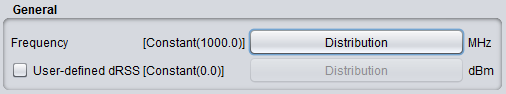Figure 68: Example of setting up the operating frequency

 

3.2.4 Transmitter

Set now the victim link transmitter by selecting the transmitter tab

Figure 74: Selecting the transmitter tab

The parameters should be filled as follows:

• The power is 30 dBm; (#1 of Figure 75)

• An omni-directional antenna of 9 dBi is used;

• The antenna height is 30 m.

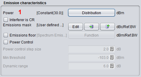
Figure 75: Example of setting up the victim link transmitter

3.2.5 Positioning the VLT vs VLR

Define now the positions of transmitters and receivers of the victim link.

Figure 76: Selecting the Tx to Rx path tab

 

SEAMCAT allows defining the locations of the Victim link receiver and the Victim link transmitter in a fixed manner (correlated) or following some distribution (uncorrelated) as summarised in Figure 77. The input parameters are detailed in section 5.4, and the algorithms are detailed in ANNEX 13:

 

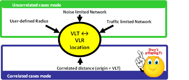
Figure 77: Summary of the VLT ↔ VLR location capability in SEAMCAT

 

In this exercise, set the distance between the VLT and the VLR as fixed (correlated distance) (x = y = 2 km) as illustrated in Figure 78. 

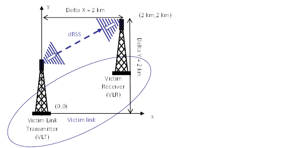
Figure 78: Distance between the Victim link transmitter and the Victim link receiver (Victim Link)

It is assumed that the Tx and Rx are both outdoor as shown in Figure 79.

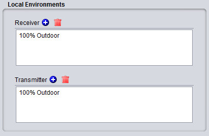
Figure 79: Example of setting up the outdoor/indoor ratio

 

For this, select the correlated distance option of SEAMCAT as shown in Figure 80. In SEAMCAT, the origin of the coverage radius (see ANNEX 13:) is the transmitter (this is also reminded in the GUI) of the link.

 

Figure 80: Illustration of the correlated distance in SEAMCAT

3.2.6 Selecting the propagation model

Since both the transmitter and the receiver characteristics and the location between the two have been defined, the propagation model needed for the simulation can be now selected.

To simplify this task, let us assume that the free space model is used to calculate the attenuation between the Victim link receiver  (VLR) and the Victim link transmitter (VLT).

In addition, the Variation should be disabled as shown in Figure 81. 

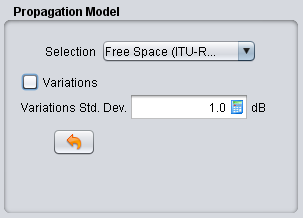
Figure 81: Example of setting up the free space propagation model for Step 1

3.2.7 Calculating the dRSS by hand

Using the Free space equation, the power received by the Victim link receiver (dRSS) can be easily derived:

  (Eq. 17)

 

Keep this calculation in mind, as it will be compared with what SEAMCAT calculates in the following sections.

3.2.8 Export/import your system to library

When setting the system is complete, it is possible to export it to the library, so it can be reused in a future point of time.

 

Figure 82: Example of importing/exporting a system to library

3.2.9 Selecting the victim in the Scenario

Now it’s time to create the victim link. The only thing needed is to select a system to be used as  victim link as shown in (#1) of Figure 83 under the “scenario” tab.

Note that the frequency field at the “scenario” tab level overwrites what was predefined at “system” tab level (#2).

 

Figure 83: Setting the system of your choice to be the victim link in the “scenario” tab

3.3 Calculating the iRSS

3.3.0 Objective

3.3.1 Interfering Links

The characteristics of the interefering system summarised in Table 7 should be entered into the SEAMCAT simulation scenario. For this example only one interfering link will be simulated.

 Table 7: Characteristics of the interfering link pair of transmitter and receiver

 

3.3.2 System to be an interferer

Contrary to the victim link, is possible to set more than one interfering link in your simulation. A given simulation workspace must contain at least one interfering link.

First edit the technical characteristics of the system(s) that will be used as interferer(s). It is possible to generate many links with the same system or with different systems. Figure 84 presents an example with 3 interfering links having each a different technical characteristic.

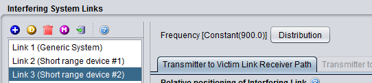
Figure 84: Example of generating multiple Interfering links

 

 

The frequency of 1000 MHz will be finally set at the “scenario” tab level (#1).

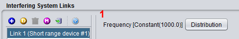
Figure 85: Setting up the operating frequency of the interfering link

3.3.3 Transmitter

Set now the victim link transmitter by selecting the transmitter tab:

• the Interefering link transmitter uses a Power of 33 dBm; (#1 of Figure 86)

• the Interefering link transmitter uses an omni-directional antenna of 11 dBi gain; (#2)

• the Interefering link transmitter uses an antenna height of 30m; (#3)

• the Interefering link transmitter uses an emission bandwidth of 200 kHz and a reference bandwidth Bref = 200 kHz. (#4)

 

The emission bandwidth of 200 kHz is defined through the emission mask (see Figure 86). This interefering link transmitter emission mask is defined in dBc. Then, enter an attenuation given in a reference bandwidth, the corresponding power is derived using the following equation:

                      (Eq.18) 

 

Where Pe is the power of the Interefering link transmitter within the emission bandwidth (also know as the in-band power). The sign of Att(dBc/Bref) is explained in section A7.5. Then, in this example, within the emission bandwidth  (200kHz- offset between –0.1 MHz and 0.1 MHz), the power is 33 dBm, if the reference bandwidth is supposed to be equal to the emission bandwidth then Att = 0 dBc/Bref, this gives:

The attenuation in dBc should be taken equal to 0 dBc/200 kHz (the link between the mask given in a reference bandwidth and the mask defined in 1 MHz is explained in ANNEX 6:).

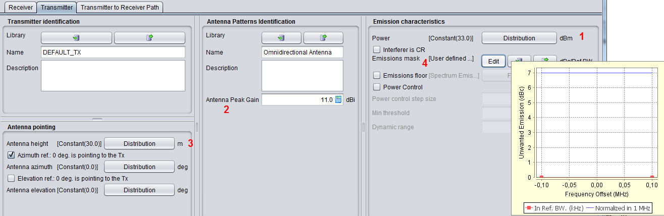
Figure 86: Setting up the interfering link transmitter

 

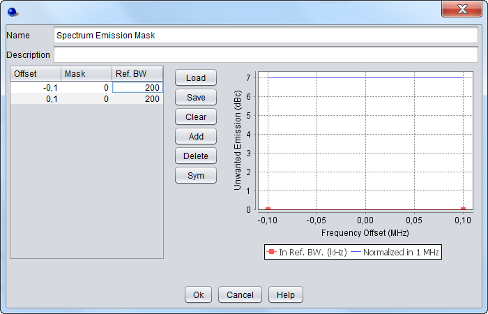
Figure 87: Spectrum emission mask settings

 

3.3.4 Receiver

For this exercise, the Power Control is not activated, therefore there is no need to fill in any information about the Interfering link receiver.

3.3.5 Positioning of the ILT vs ILR

Positioning of the ILT vs ILR is similar to positioning VLT vs VLR as described in Section 3.2.5.

This is required when the power control in the interfering link is simulated. It is also important to set it in case the geometry of the scenario is dependant on the position of the ILR (for instance ILR being at the center of the ILT distribution, or the victim link being fixed with respect to the ILR).

3.3.6 Positioning of the VLR vs ILT

SEAMCAT allows defining the relative location between the Victim link receiver and the Interefering link transmitter as illustrated in Figure 88. The input parameters are detailed in section 10.3, and the algorithms are detailed in ANNEX 13:

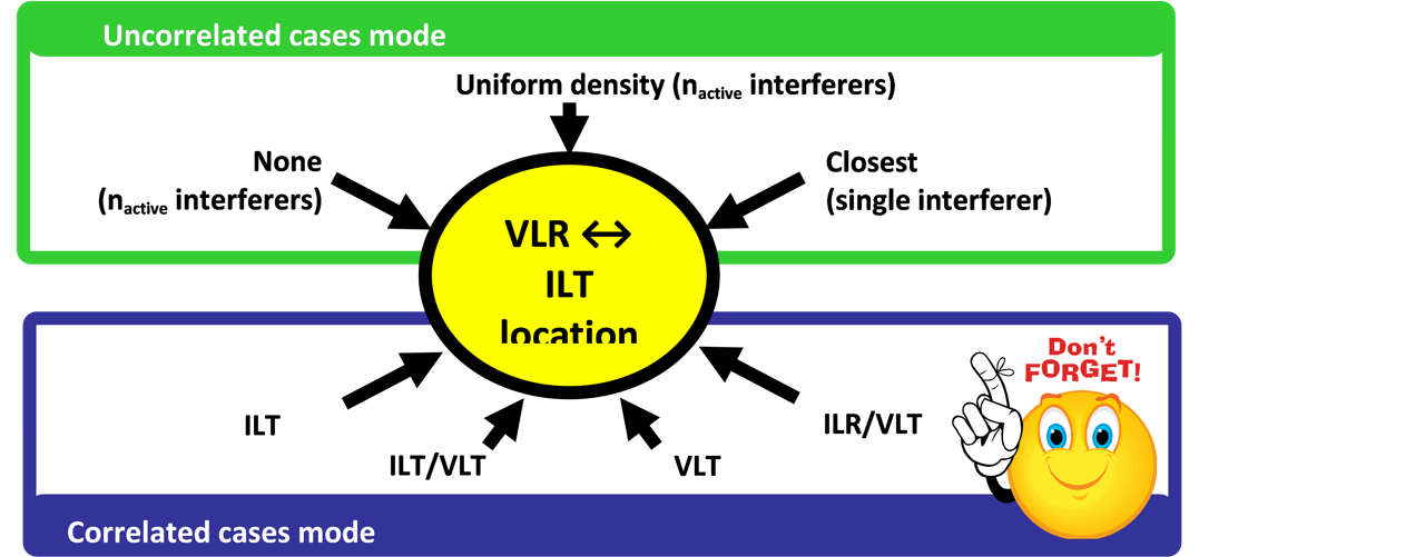
Figure 88: Summary of the VLR ↔ ILT location capability in SEAMCAT

 

In this exercise, the distance between the Interefering link transmitter and the Victim link receiver as shown in Figure 89 is fixed by using the correlated distance as illustrated by Figure 90. 

 

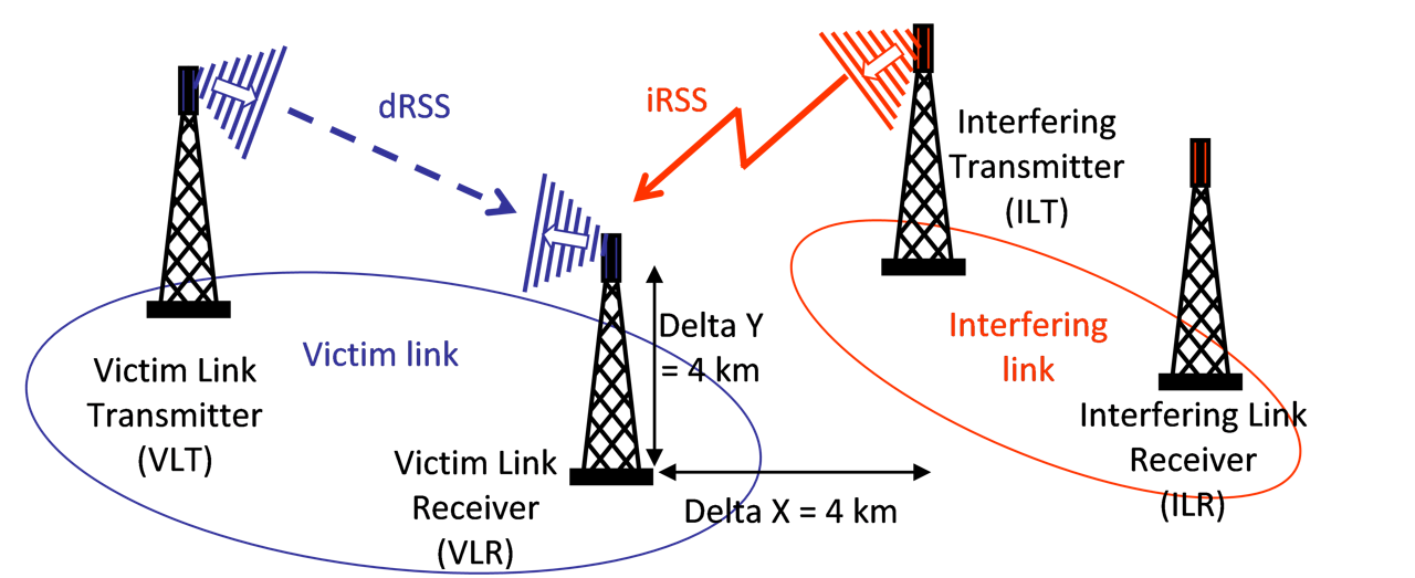
Figure 89: Distance between the Interefering link transmitter and the Victim link receiver 

 

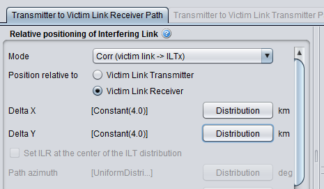
Figure 90: Excample of setting up the distance between the Interefering link transmitter and the Victim link receiver in SEAMCAT. Here the ILT is positioned relative to the VLR

3.3.7 Calculating the iRSS by hand

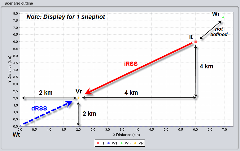
Figure 91: Illustration of SEAMCAT display (only 1 snapshot) of the various pair of transmitter and receiver and the dRSS and iRSS relationship

The attenuation between the Interefering link transmitter and the Victim link receiver is simulated by using the free space model (Variation should be disabled). When the simulation is finished, SEAMCAT presents the positioning of the various pairs of transmitters and receivers as shown in Figure 91(only one snapshot is illustrated).

Using these assumptions, it is possible to derive the interfering power received by the Victim link receiver iRSS:

(Eq.19)

 

3.3.8 Emission, reference, VLR bandwidth relationship and bandwidth correction factor

The proposed exercise considers the case where the VLR bandwidth is the same as the emission bandwidth and the reference bandwidth. 

This section aims at illustrating the interaction between the emission bandwidth (It_BW), reference bandwidth (Bref), VLR bandwidth (VLR_BW) and any bandwidth correction factor. This section provides examples where these values are different and its’ effect on the iRSS calculation.

 

Relationship between Emission bandwidth and Reference bandwidth

For a fixed VLR_BW = 200 kHz, and fixed It_BW= 200 kHz, the attenuation Att(dBc/Bref) will be different depending on the values of the Bref in order to achieve the same interference power level.

Case 1, It_BW > Bref :

Bref = 100 kHz, with Att = -3 dBc/Bref, iRSS =  -54.49 dBm;                                           

 

As mentioned in Section A7.5 on p.287, if the reference bandwidth is lower than the emission bandwidth then the attenuation must be defined with negative sign;

Case 2, It_BW = Bref:

Bref = 200 kHz, with Att = 0 dBc/Bref, iRSS =  -54.49 dBm;                                            

 

If the reference bandwidth is equal to the emission bandwidth then the attenuation should be set  as zero.

 

Case 3, It_BW < Bref:

Bref = 400 kHz, with Att = 3 dBc/Bref, iRSS =  -54.49 dBm;                                             

 

If the reference bandwidth is larger than the emission bandwidth then the attenuation must be defined with positive sign.

 

Please note that, it is best practice and recommended that the user set the reference bandwidth as the same value as the bandwidth of the emission mask, to avoid any unexpected scaling effect.

 

 

Relationship between Emission bandwidth and Victim link receiver bandwidth

For a fixed Bref = 200 kHz and a fixed It_BW= 200 kHz, depending on the size of the VLR_BW a bandwidth correction factor is applied or not. Calculations presented here are mainly illustration of effect or relation between emission Bw nad VLR Bw in the co-frequency case.

 

Case 4, It_BW = VLR_BW:

VLR_BW = 200 kHz, iRSS =  -54.49 dBm;                                                             

 

Case 5, It_BW > VLR_BW:

VLR_BW = 100 kHz, iRSS =  -57.5 dBm;                                                               

As shown in ANNEX 22: on p. 422, when the It_BW > VLR_BW, the interfering power in the VLR is reduced due a bandwidth correction factor automatically applied in SEAMCAT. As a results, the iRSS value decreases compare to a case where It_BW = VLR_BW.

 

Case 6, It_BW < VLR_BW:  Case of ILT Spectrum emission mask when the Tx spectrum is sharply reduced outside its reference bandwidth

VLR_BW = 400 kHz, iRSS =  -54.49 dBm;                                                             

As illustrated in ANNEX 22:, when the It_BW < VLR_BW, there is no bandwidth correction factor applied to the interfering emitted power since the all the energy is “seen” by the VLR. Therefore the iRSS is equal to the case where It_BW = VLR_BW. Note also that since the emission bandwidth of the interferer is smaller than the victim, SEAMCAT will complain that the spectrum emission mask of the interferer is not defined with the range of the victim bandwidth, therefore you need to increase the out of band emission.

 

 

Case 7: It_BW < VLR_BW: Case of ILT Spectrum emission mask when the Tx spectrum have sloped characteristics outside its reference bandwidth

This is the same as case 6 (VLR = 400 kHz and Bref = 200 kHz) except that the  spectrum emission mask (emission bandwidth 200 kHz) has slopes on both sides (Figure 93) which generates higher interference compared to the case 6  and the iRSS = -53.44 dBm

 

3.4 Launching a simulation

A simulation is now ready to be launched. It should be noted that prior to beginning the simulation, SEAMCAT checks the consistency and suitability of certain input parameters (see ANNEX 19:).

Since the default operating frequency of the Interfering link transmitter is 900 MHz and the unwanted emission mask is not within the range of the Victim link receiver, SEAMCAT automatically complains and displays a warning window.

 

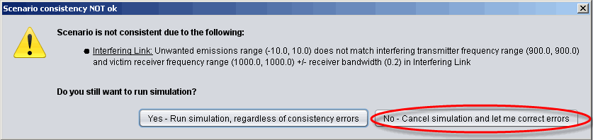
Therefore, it’s better to select “No - Cancel simulation and let me correct errors” and define the operating frequency (1000 MHz) of the interfering link. These parameters do not affect the calculation of the dRSS. It is only to ensure that SEAMCAT does not experience any exceptions when running.

3.5 Extract results vectors (dRSS, iRSS etc...)

You can extract the dRSS vectors from the “Results” panel in the newly create workspace results in Figure 95

 

 

 

 

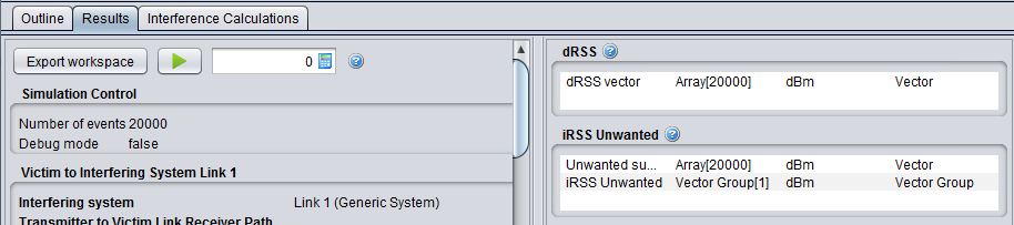
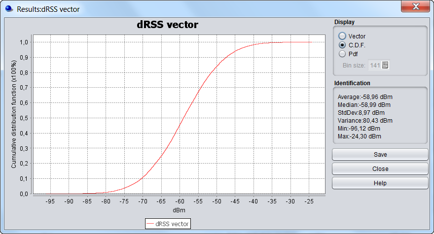
When double clicking on a result vector field (Figure 36 (#1)) the display panel as shown in Figure 96, offers three options to display the results in vector (limited to 20.000 events), CDF and PDF format. 

In addition, some statistical information can be displayed such as average, median, standard deviation (StdDev), variance, min and max. Further information about these statistics (i.e. how they are computed) are to be found in Section A1.5.

3.6 Calculating the probability of interference

Objective

 

After the simulation of all events has completed, SEAMCAT will have calculated and stored the dRSS and iRSS vectors. Now it is possible to evaluate the probability of interference for the simulated scenario using the interference calculation control panel as shown in Figure 97.

 

 

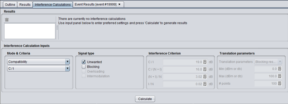
Any of the following parameters can be selected from the panel when calculating the probability of interference: 

• Calculation mode: compatibility or translation;

• Which type of interference signal is considered for calculation: unwanted, blocking, overloading, intermodulation or a combination of them;

• Interference criterion: C/I, C/(N+I), (N+I)/N or I/N:

 

3.6.1 Compatibility calculation mode

It is then possible to derive the C/I (i.e. dRSS/iRSS equivalent to dRSS-iRSS in dB):

dRSS/iRSS = -53.5-(-54.5) = 1 dB                                                

Since the resulting C/I is below the protection criteria (19 dB), the probability of interference calculated by SEAMCAT (compatibility calculation mode) is equal to 1 as shown in Figure 98

3.6.2 Translation calculation mode

When the Translation mode is chosen, it is possible to calculate and display a chart of the probability of interference as a function of one of the following input parameters:

• Output power of Interefering link transmitter;

• Blocking response level of Victim link receiver;

• Intermodulation response level of Victim link receiver.

 

The translation function, as shown as (#1) Figure 98 in, allows investigation of the probability of interference for varying power supplied (#2) to the interefering link transmitter. The power supplied (#3) to the interfering link transmitter should be equal to 15 dBm, which is 18 dB below the value used in the simulation (33 dBm). Effectively the C/I will be increased by 18 dB and reaches the level of 19 dB.

 

Figure 98: Translation function

3.6.3 Example of probability of interference calculation

The protection criteria to be used for the calculation of the probability of interference and the type of interference to be considered (unwanted and/or blocking) can be equally chosen (see Figure 97).

 

Using the unwanted mode, it is possible to derive the C/I:

dRSS/iRSS_unwanted = -53.5- (-77.5) = 24 dB

 

Since the resulting C/I is above the protection criteria (19 dB), the probability of interference calculated by SEAMCAT (Interference calculation) is equal to 0).

 

The same conclusion is reached by using the C/(N+I) criteria. It should be noted that SEAMCAT performs a consistency check (ANNEX 19:) between the interference criteria (ANNEX 3:).

 

It is also possible to derive the (N+I)/N= -77.5-(-100)= 22.5 (since I>>N). Since the (I+N)/N which is obtained is above the protection criteria (3 dB), the probability of interference calculated by SEAMCAT (Interference calculation) is equal to 1).

The same conclusion is reached by using the I/N criteria.

 

Using the blocking interference mode (protection ratio) it is then possible to derive the C/I:

 

dRSS/iRSS_blocking = -53.5 - (-113.5) = 60 dB

 

Since the C/I obtained is above the protection criteria (19 dB), the probability of interference calculated by SEAMCAT (Interference calculation) is equal to 0).

 

It is also possible to derive the (N+I)/N= -113.5-(-100)= -13.5. Since the (N+I)/N which is obtained is below the protection criteria (3 dB), the probability of interference calculated by SEAMCAT (Interference calculation) is equal to 0).

 

Then, by taking into account the sum of the two signal types, the probability of interference becomes equal to 1 (due to the unwanted emissions)