# 3.3 Calculating the iRSS

# 3.3.0 Objective

[![image.png](https://wiki.cept.org/uploads/images/gallery/2026-04/scaled-1680-/9zVg4kz0BCSu8ziI-image.png)](https://wiki.cept.org/uploads/images/gallery/2026-04/9zVg4kz0BCSu8ziI-image.png)

# 3.3.1 Interfering Links

The characteristics of the interefering system summarised in Table 7 should be entered into the SEAMCAT simulation scenario. For this example only one interfering link will be simulated.

 Table 7: Characteristics of the interfering link pair of transmitter and receiver**

<div class="pm-table-container with-shadow-observer" data-layout="align-start" data-testid="table-container" id="bkmrk-parameters-value-uni"><div class="pm-table-wrapper" data-autosize="false" data-layout="align-start" data-number-column="false" data-table-local-id="" data-vc="table-node-wrapper"><div class="sentinel-left"></div><table data-layout="align-start" data-number-column="false" data-table-width="760" data-testid="renderer-table"><colgroup></colgroup><tbody><tr><td colspan="1" rowspan="1">Parameters

</td><td colspan="1" rowspan="1">Value

</td><td colspan="1" rowspan="1">Units

</td></tr><tr><td colspan="1" rowspan="1">Operating frequency

</td><td colspan="1" rowspan="1">1000

</td><td colspan="1" rowspan="1">MHz

</td></tr><tr><td colspan="1" rowspan="1">Transmitter power

</td><td colspan="1" rowspan="1">33

</td><td colspan="1" rowspan="1">dBm

</td></tr><tr><td colspan="1" rowspan="1">Emission bandwidth

</td><td colspan="1" rowspan="1">200

</td><td colspan="1" rowspan="1">kHz

</td></tr><tr><td colspan="1" rowspan="1">Reference bandwidth

</td><td colspan="1" rowspan="1">200

</td><td colspan="1" rowspan="1">kHz

</td></tr><tr><td colspan="1" rowspan="1">Tx antenna type

</td><td colspan="1" rowspan="1">Omni directional

</td><td colspan="1" rowspan="1"></td></tr><tr><td colspan="1" rowspan="1">Tx antenna gain

</td><td colspan="1" rowspan="1">11

</td><td colspan="1" rowspan="1">dBi

</td></tr><tr><td colspan="1" rowspan="1">Tx antenna height

</td><td colspan="1" rowspan="1">30

</td><td colspan="1" rowspan="1">m

</td></tr></tbody></table>

<div class="sentinel-right">  
</div></div><div class="pm-table-sticky-scrollbar-container-view-page" data-vc="table-sticky-scrollbar-container"><div>  
</div></div><div class="pm-table-sticky-scrollbar-sentinel-bottom" data-testid="sticky-scrollbar-sentinel-bottom">  
</div></div>

# 3.3.2 System to be an interferer

Contrary to the victim link, is possible to set more than one interfering link in your simulation. A given simulation workspace must contain at least one interfering link.

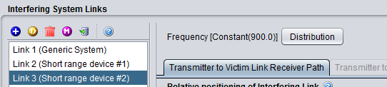
First edit the technical characteristics of the system(s) that will be used as interferer(s). It is possible to generate many links with the same system or with different systems. Figure 84 presents an example with 3 interfering links having each a different technical characteristic.

[![image.png](https://wiki.cept.org/uploads/images/gallery/2026-04/scaled-1680-/tBtCErxC9uSLLdwu-image.png)](https://wiki.cept.org/uploads/images/gallery/2026-04/tBtCErxC9uSLLdwu-image.png)

**Figure 84: Example of generating multiple Interfering links**

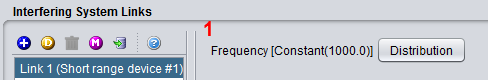
The frequency of 1000 MHz will be finally set at the “scenario” tab level (**\#1**).

[![image.png](https://wiki.cept.org/uploads/images/gallery/2026-04/scaled-1680-/B4cZ7u63ne1yU7w1-image.png)](https://wiki.cept.org/uploads/images/gallery/2026-04/B4cZ7u63ne1yU7w1-image.png)

**Figure 85: Setting up the operating frequency of the interfering link**

# 3.3.3 Transmitter

Set now the victim link transmitter by selecting the transmitter tab:

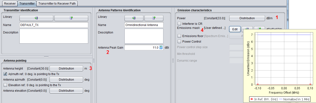
- the Interefering link transmitter uses a Power of 33 dBm; (**\#1** of Figure 86)
- the Interefering link transmitter uses an omni-directional antenna of 11 dBi gain; (**\#2**)
- the Interefering link transmitter uses an antenna height of 30m; (**\#3**)
- the Interefering link transmitter uses an emission bandwidth of 200 kHz and a reference bandwidth Bref = 200 kHz. (**\#4**)

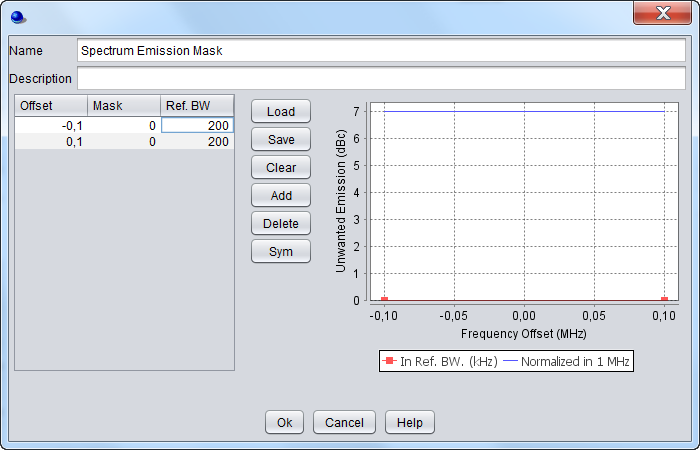
The emission bandwidth of 200 kHz is defined through the emission mask (see Figure 86). This interefering link transmitter emission mask is defined in dBc. Then, enter an attenuation given in a reference bandwidth, the corresponding power is derived using the following equation:

![image.png](https://wiki.cept.org/uploads/images/gallery/2026-04/scaled-1680-/lx6pBRnEVWEKSMt3-image.png) (Eq.18)

Where Pe is the power of the Interefering link transmitter within the emission bandwidth (also know as the in-band power). The sign of Att(dBc/Bref) is explained in section A7.5. Then, in this example, within the emission bandwidth (200kHz- offset between –0.1 MHz and 0.1 MHz), the power is 33 dBm, if the reference bandwidth is supposed to be equal to the emission bandwidth then Att = 0 dBc/Bref, this gives:

![image.png](https://wiki.cept.org/uploads/images/gallery/2026-04/scaled-1680-/exMJxbq8VCmGbdMq-image.png)

The attenuation in dBc should be taken equal to 0 dBc/200 kHz (the link between the mask given in a reference bandwidth and the mask defined in 1 MHz is explained in ANNEX 6:).

[![image.png](https://wiki.cept.org/uploads/images/gallery/2026-04/scaled-1680-/KBa2lkVSnE8b8WZ9-image.png)](https://wiki.cept.org/uploads/images/gallery/2026-04/KBa2lkVSnE8b8WZ9-image.png)

**Figure 86: Setting up the interfering link transmitter**

[![image.png](https://wiki.cept.org/uploads/images/gallery/2026-04/scaled-1680-/MRGXFCW2XfZw8t6Z-image.png)](https://wiki.cept.org/uploads/images/gallery/2026-04/MRGXFCW2XfZw8t6Z-image.png)

**Figure 87: Spectrum emission mask settings**

# 3.3.4 Receiver

For this exercise, the Power Control is not activated, therefore there is no need to fill in any information about the Interfering link receiver.

# 3.3.5 Positioning of the ILT vs ILR

Positioning of the <span data-highlighted="true" data-vc="highlighted-text"><span class="_kqswh2mm"><span class="_5pioz8co _189e1dm9 _1il9buyh _19lc184f _d0altlke" data-testid="definition-highlighter">ILT</span></span></span> vs <span data-highlighted="true" data-vc="highlighted-text"><span class="_kqswh2mm"><span class="_5pioz8co _189e1dm9 _1il9buyh _19lc184f _d0altlke" data-testid="definition-highlighter">ILR</span></span></span> is similar to positioning <span data-highlighted="true" data-vc="highlighted-text"><span class="_kqswh2mm"><span class="_5pioz8co _189e1dm9 _1il9buyh _19lc184f _d0altlke" data-testid="definition-highlighter">VLT</span></span></span> vs <span data-highlighted="true" data-vc="highlighted-text"><span class="_kqswh2mm"><span class="_5pioz8co _189e1dm9 _1il9buyh _19lc184f _d0altlke" data-testid="definition-highlighter">VLR</span></span></span> as described in Section 3.2.5.

This is required when the power control in the interfering link is simulated. It is also important to set it in case the geometry of the scenario is dependant on the position of the <span data-highlighted="true" data-vc="highlighted-text">ILR</span> (for instance <span data-highlighted="true" data-vc="highlighted-text">ILR</span> being at the center of the <span data-highlighted="true" data-vc="highlighted-text">ILT</span> distribution, or the victim link being fixed with respect to the <span data-highlighted="true" data-vc="highlighted-text">ILR</span>).

# 3.3.6 Positioning of the VLR vs ILT

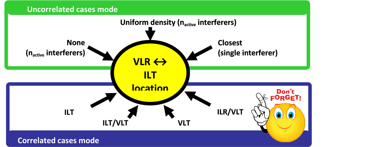
SEAMCAT allows defining the relative location between the Victim link receiver and the Interefering link transmitter as illustrated in Figure 88. The input parameters are detailed in section 10.3, and the algorithms are detailed in ANNEX 13:

[![image.png](https://wiki.cept.org/uploads/images/gallery/2026-04/scaled-1680-/zRpf5jmmg1py9uIn-image.png)](https://wiki.cept.org/uploads/images/gallery/2026-04/zRpf5jmmg1py9uIn-image.png)

**Figure 88: Summary of the <span data-highlighted="true" data-vc="highlighted-text"><span class="_kqswh2mm"><span class="_5pioz8co _189e1dm9 _1il9buyh _19lc184f _d0altlke" data-testid="definition-highlighter">VLR</span></span></span> ↔ <span data-highlighted="true" data-vc="highlighted-text"><span class="_kqswh2mm"><span class="_5pioz8co _189e1dm9 _1il9buyh _19lc184f _d0altlke" data-testid="definition-highlighter">ILT</span></span></span> location capability in SEAMCAT**

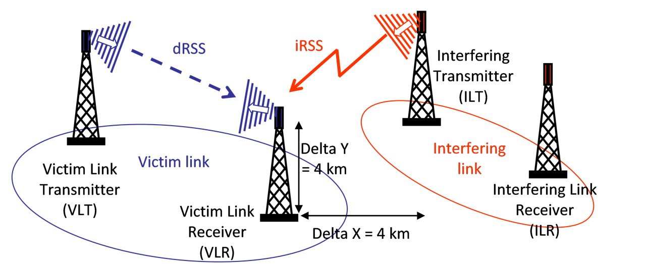
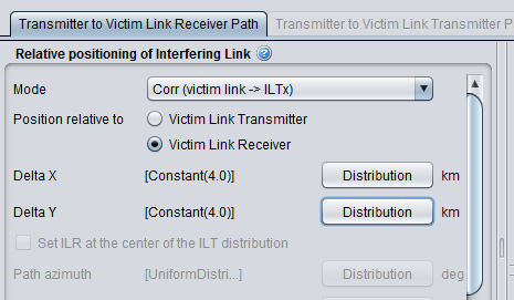
In this exercise, the distance between the Interefering link transmitter and the Victim link receiver as shown in Figure 89 is fixed by using the correlated distance as illustrated by Figure 90.

[![image.png](https://wiki.cept.org/uploads/images/gallery/2026-04/scaled-1680-/1UAV0eK3Ejs29Wly-image.png)](https://wiki.cept.org/uploads/images/gallery/2026-04/1UAV0eK3Ejs29Wly-image.png)

**Figure 89: Distance between the Interefering link transmitter and the Victim link receiver**

[![image.png](https://wiki.cept.org/uploads/images/gallery/2026-04/scaled-1680-/KRZ3SV5GjPX7dgbm-image.png)](https://wiki.cept.org/uploads/images/gallery/2026-04/KRZ3SV5GjPX7dgbm-image.png)

**Figure 90: Excample of setting up the distance between the Interefering link transmitter and the Victim link receiver in SEAMCAT. Here the <span data-highlighted="true" data-vc="highlighted-text">ILT</span> is positioned relative to the <span data-highlighted="true" data-vc="highlighted-text">VLR</span>**

# 3.3.7 Calculating the iRSS by hand

[![image.png](https://wiki.cept.org/uploads/images/gallery/2026-04/scaled-1680-/zZN7g8sxgSI5UyrN-image.png)
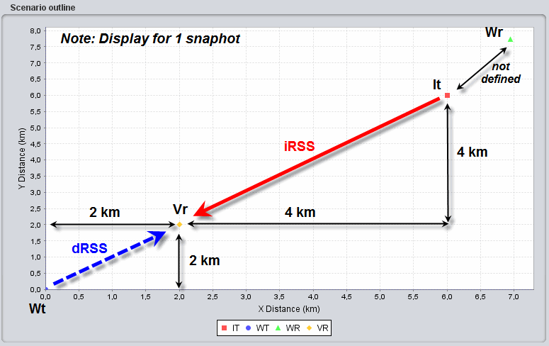
](https://wiki.cept.org/uploads/images/gallery/2026-04/zZN7g8sxgSI5UyrN-image.png)

**Figure 91: Illustration of SEAMCAT display (only 1 snapshot) of the various pair of transmitter and receiver and the dRSS and iRSS relationship**

The attenuation between the Interefering link transmitter and the Victim link receiver is simulated by using the free space model (Variation should be disabled). When the simulation is finished, SEAMCAT presents the positioning of the various pairs of transmitters and receivers as shown in Figure 91(only one snapshot is illustrated).

Using these assumptions, it is possible to derive the interfering power received by the Victim link receiver iRSS:

(Eq.19)

[![image.png](https://wiki.cept.org/uploads/images/gallery/2026-04/scaled-1680-/XkoNhOMOROWh5ee2-image.png)](https://wiki.cept.org/uploads/images/gallery/2026-04/XkoNhOMOROWh5ee2-image.png)

[![image.png](https://wiki.cept.org/uploads/images/gallery/2026-04/scaled-1680-/DfMreHzs8u6etA8i-image.png)](https://wiki.cept.org/uploads/images/gallery/2026-04/DfMreHzs8u6etA8i-image.png)

[![image.png](https://wiki.cept.org/uploads/images/gallery/2026-04/scaled-1680-/gdZzXXIXnuGhiMOF-image.png)](https://wiki.cept.org/uploads/images/gallery/2026-04/gdZzXXIXnuGhiMOF-image.png)

# 3.3.8 Emission, reference, VLR bandwidth relationship and bandwidth correction factor

The proposed exercise considers the case where the <span data-highlighted="true" data-vc="highlighted-text"><span class="_kqswh2mm"><span class="_5pioz8co _189e1dm9 _1il9buyh _19lc184f _d0altlke" data-testid="definition-highlighter">VLR</span></span></span> bandwidth is the same as the emission bandwidth and the reference bandwidth.

This section aims at illustrating the interaction between the emission bandwidth (It<sub data-renderer-mark="true">BW</sub>), reference bandwidth (Bref), <span data-highlighted="true" data-vc="highlighted-text">VLR</span> bandwidth (<span data-highlighted="true" data-vc="highlighted-text">VLR</span><sub data-renderer-mark="true">BW</sub>) and any bandwidth correction factor. This section provides examples where these values are different and its’ effect on the iRSS calculation.

### Relationship between Emission bandwidth and Reference bandwidth

For a fixed VLR<sub data-renderer-mark="true">BW</sub> = 200 kHz, and fixed It<sub data-renderer-mark="true">BW</sub>= 200 kHz, the attenuation Att(dBc/Bref) will be different depending on the values of the Bref in order to achieve the same interference power level.

 **Case 1, It<sub data-renderer-mark="true">BW</sub> &gt; Bref :**

Bref = 100 kHz, with Att = -3 dBc/Bref, iRSS = -54.49 dBm;

As mentioned in Section A7.5 on p.287, if the reference bandwidth is lower than the emission bandwidth then the attenuation must be defined with negative sign;

 **Case 2, It<sub data-renderer-mark="true">BW</sub> = Bref:**

Bref = 200 kHz, with Att = 0 dBc/Bref, iRSS = -54.49 dBm;

If the reference bandwidth is equal to the emission bandwidth then the attenuation should be set as zero.

**Case 3, It<sub data-renderer-mark="true">BW</sub> &lt; Bref:**

Bref = 400 kHz, with Att = 3 dBc/Bref, iRSS = -54.49 dBm;

If the reference bandwidth is larger than the emission bandwidth then the attenuation must be defined with positive sign.

Please note that, it is best practice and recommended that the user set the reference bandwidth as the same value as the bandwidth of the emission mask, to avoid any unexpected scaling effect.

### Relationship between Emission bandwidth and Victim link receiver bandwidth

  
For a fixed Bref = 200 kHz and a fixed It<sub data-renderer-mark="true">BW</sub>= 200 kHz, depending on the size of the <span data-highlighted="true" data-vc="highlighted-text"><span class="_kqswh2mm"><span class="_5pioz8co _189e1dm9 _1il9buyh _19lc184f _d0altlke" data-testid="definition-highlighter">VLR</span></span></span><sub data-renderer-mark="true">BW</sub> a bandwidth correction factor is applied or not. Calculations presented here are mainly illustration of effect or relation between emission Bw nad <span data-highlighted="true" data-vc="highlighted-text">VLR</span> Bw in the co-frequency case.

**Case 4, It<sub data-renderer-mark="true">BW</sub> = <span data-highlighted="true" data-vc="highlighted-text">VLR</span><sub data-renderer-mark="true">BW</sub>:**

<span data-highlighted="true" data-vc="highlighted-text">VLR</span>**<sub data-renderer-mark="true">BW</sub>** = 200 kHz, iRSS = -54.49 dBm;

**Case 5, It<sub data-renderer-mark="true">BW</sub> &gt; <span data-highlighted="true" data-vc="highlighted-text">VLR</span><sub data-renderer-mark="true">BW</sub>:**

<span data-highlighted="true" data-vc="highlighted-text">VLR</span>**<sub data-renderer-mark="true">BW</sub>** = 100 kHz, iRSS = -57.5 dBm;

As shown in ANNEX 22: on p. 422, when the It<sub data-renderer-mark="true">BW</sub> &gt; <span data-highlighted="true" data-vc="highlighted-text">VLR</span><sub data-renderer-mark="true">BW</sub>, the interfering power in the <span data-highlighted="true" data-vc="highlighted-text">VLR</span> is reduced due a bandwidth correction factor automatically applied in SEAMCAT. As a results, the iRSS value decreases compare to a case where It<sub data-renderer-mark="true">BW</sub> = <span data-highlighted="true" data-vc="highlighted-text">VLR</span><sub data-renderer-mark="true">BW</sub>.

**Case 6, It<sub data-renderer-mark="true">BW</sub> &lt; <span data-highlighted="true" data-vc="highlighted-text">VLR</span><sub data-renderer-mark="true">BW</sub>: Case of <span data-highlighted="true" data-vc="highlighted-text"><span class="_kqswh2mm"><span class="_5pioz8co _189e1dm9 _1il9buyh _19lc184f _d0altlke" data-testid="definition-highlighter">ILT</span></span></span> Spectrum emission mask when the Tx spectrum is sharply reduced outside its reference bandwidth**

<span data-highlighted="true" data-vc="highlighted-text">VLR</span>**<sub data-renderer-mark="true">BW</sub>** = 400 kHz, iRSS = -54.49 dBm;

As illustrated in ANNEX 22:, when the It<sub data-renderer-mark="true">BW</sub> &lt; <span data-highlighted="true" data-vc="highlighted-text">VLR</span><sub data-renderer-mark="true">BW</sub>, there is no bandwidth correction factor applied to the interfering emitted power since the all the energy is “seen” by the <span data-highlighted="true" data-vc="highlighted-text">VLR</span>. Therefore the iRSS is equal to the case where It<sub data-renderer-mark="true">BW</sub> = <span data-highlighted="true" data-vc="highlighted-text">VLR</span><sub data-renderer-mark="true">BW</sub>. Note also that since the emission bandwidth of the interferer is smaller than the victim, SEAMCAT will complain that the spectrum emission mask of the interferer is not defined with the range of the victim bandwidth, therefore you need to increase the out of band emission.

![image.png](https://wiki.cept.org/uploads/images/gallery/2026-04/scaled-1680-/4DUlngx0BBFvFUDH-image.png)

<div class="rich-media-item mediaSingleView-content-wrap image-align-start css-17voqo2" data-layout="align-start" data-media-vc-wrapper="true" data-node-type="mediaSingle" data-renderer-start-pos="1516" data-vc="media-single" data-width="554" data-width-type="pixel" id="bkmrk-figure-92%3A-illustrat"><div class="css-110bcf8"><div data-alt="" data-collection="contentId-493565" data-context-id="493565" data-file-mime-type="" data-file-name="file" data-file-size="1" data-height="318" data-id="787351f4-8a39-432d-ae93-99c33ec84cc7" data-node-type="media" data-renderer-start-pos="1517" data-type="file" data-width="705"><div class="_2rko18qm _vchhusvi _kqswh2mm _ect4ttxp _p12f1osq _c71l1osq _1bsb1qmm _4t3ine4n _1hlmd0i9 _1rquusvi _eg541i5c _mts3kb7n _1ntskb7n _yfmhtlke _5sb1v00u new-file-experience-wrapper" data-media-vc-wrapper="true" data-testid="media-card-view" id="bkmrk-figure-92%3A-illustrat-1"><div class="_1reo15vq _18m915vq _2rko18qm _1e0c1txw _kqswh2mm _p12f1osq _1bsb1osq _4t3i1osq _c71l1osq media-file-card-view" data-cursor="pointer" data-test-media-name="92.png" data-test-progress="1" data-test-source="remote" data-test-status="complete" data-testid="media-file-card-view"><div class="_kqswstnw _1bsb1osq _4t3i1osq _1e0c1txw _2lx21bp4 _1bah1h6o _4cvr1h6o align-center" data-testid="ImageRendererWrapper">![](blob:https://ecowiki.atlassian.net/ba4e46a1-2ea8-4e46-8903-301b5794a9f0#media-blob-url=true&id=787351f4-8a39-432d-ae93-99c33ec84cc7&collection=contentId-493565&contextId=493565&width=705&height=318&alt=&clientId=113268fe-fe5b-4bc3-8ff3-07965dbf1d18)**
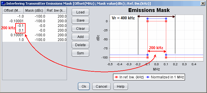
Figure 92: Illustration of the emission spectrum mask with respect to the <span data-highlighted="true" data-vc="highlighted-text">VLR</span> bandwidth in case 6**</div></div></div></div></div></div>**Case 7: It<sub data-renderer-mark="true">BW</sub> &lt; <span data-highlighted="true" data-vc="highlighted-text">VLR</span><sub data-renderer-mark="true">BW</sub>: Case of <span data-highlighted="true" data-vc="highlighted-text">ILT</span> Spectrum emission mask when the Tx spectrum have sloped characteristics outside its reference bandwidth**

This is the same as case 6 (<span data-highlighted="true" data-vc="highlighted-text">VLR</span> = 400 kHz and Bref = 200 kHz) except that the spectrum emission mask (emission bandwidth 200 kHz) has slopes on both sides (Figure 93) which generates higher interference compared to the case 6 and the iRSS = -53.44 dBm

![image.png](https://wiki.cept.org/uploads/images/gallery/2026-04/scaled-1680-/kNI3Nt4H85sjWgTu-image.png)

<div class="rich-media-item mediaSingleView-content-wrap image-align-start css-lyf5b2" data-layout="align-start" data-media-vc-wrapper="true" data-node-type="mediaSingle" data-renderer-start-pos="2015" data-vc="media-single" data-width="553" data-width-type="pixel" id="bkmrk-figure-93%3A-illustrat"><div class="css-5mfdbi"><div data-alt="" data-collection="contentId-493565" data-context-id="493565" data-file-mime-type="" data-file-name="file" data-file-size="1" data-height="320" data-id="2ad47554-6a2d-4112-83aa-771c4b124652" data-node-type="media" data-renderer-start-pos="2016" data-type="file" data-width="708"><div class="_2rko18qm _vchhusvi _kqswh2mm _ect4ttxp _p12f1osq _c71l1osq _1bsb1qmm _4t3ine4n _1hlmd0i9 _1rquusvi _eg541i5c _mts3kb7n _1ntskb7n _yfmhtlke _5sb1v00u new-file-experience-wrapper" data-media-vc-wrapper="true" data-testid="media-card-view" id="bkmrk-figure-93%3A-illustrat-1"><div class="_1reo15vq _18m915vq _2rko18qm _1e0c1txw _kqswh2mm _p12f1osq _1bsb1osq _4t3i1osq _c71l1osq media-file-card-view" data-cursor="pointer" data-test-media-name="93.png" data-test-progress="1" data-test-source="remote" data-test-status="complete" data-testid="media-file-card-view"><div class="_kqswstnw _1bsb1osq _4t3i1osq _1e0c1txw _2lx21bp4 _1bah1h6o _4cvr1h6o align-center" data-testid="ImageRendererWrapper">![](blob:https://ecowiki.atlassian.net/b43c5056-41ab-4454-9186-c12fbce8fe5a#media-blob-url=true&id=2ad47554-6a2d-4112-83aa-771c4b124652&collection=contentId-493565&contextId=493565&width=708&height=320&alt=&clientId=113268fe-fe5b-4bc3-8ff3-07965dbf1d18)**
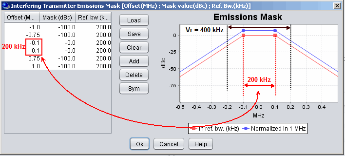
Figure 93: Illustration of case 7 and the “extra” interfering energy to the <span data-highlighted="true" data-vc="highlighted-text">VLR</span> due to**   
 **the slope in the emission mask**</div></div></div></div></div></div>