2. Getting around in SEAMCAT

• 2.1 Quick buttons toolbar
• 2.2 Welcome to SEAMCAT window
• 2.3 Typical SEAMCAT workflow
• 2.4 Simulation Workspace
• 2.4.1 Scenario workspace
• 2.4.2 Results workspace
• 2.5 Create or update a simulation workspace
• 2.6 Batch operation
• 2.7 Running and stopping a simulation
• 2.8 Running from the command line
• 2.9 Consistency check
• 2.10 Simulation control
• 2.11 Simulation results overview
• 2.12 Saving options in SEAMCAT
• 2.12.1 Saving workspace and batch
• 2.12.2 Saving results - file extension
• 2.13 Simulation report
• 2.14 Logging function for debugging
• 2.15 Play / Replay an event
• 2.16 Testing propagation models
• 2.17 Testing distribution functions
• 2.18 Testing unwanted emissions function
• 2.19 Multiple vectors comparison
• 2.20 Pocket calculator
• 2.21 Online manual and help content
• 2.22 Report enhancements and bugs
• 2.23 Installing plugins in SEAMCAT
• 2.24 Pausing and RESUMING a simulation
• 2.25 Considering time domain Tx activity
• Methods for applying time-domain activity of transmissions in SEAMCAT simulation

2.1 Quick buttons toolbar

A ‘quick buttons’ toolbar with access to the most commonly used features is avaialable at the top of the SEAMCAT interface window. The function of each button is shown in a tooltip whenever your mouse is moved over it. Certain  buttons are inactive when the function is not applicable, e.g. the stop simulation button is active only during the run of a simulation. Inactive buttons are displayed dimmed.

 

 

2.2 Welcome to SEAMCAT window

Every time SEAMCAT is launched, a welcome dialog box is displayed which allows the selection of various options (the welcome dialog box can be disabled under File/Configuration). The first step is typically to create a new workspace or open a previously created workspace. This is done by selecting ‘New’, ‘Open’ or ‘Recently Used’ (to open the most recent workspaces from the displayed list). ‘New Batch’ can be used to specify multiple sequential simulation runs using new or existing workspaces. ‘Calc’ launches the SEAMCAT calculator which is a convenient tool for common basic engineering calculations.

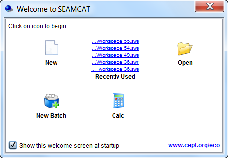
Figure 19: Welcome pop up window

When a new workspace is created, it will initially be automatically assigned a name 'Workspace xyz', where xyz is the serial number of the newly created workspace. The workspace name may be changed at any time afterwards using Save or Save As. The file in your file system can also be renamed - SEAMCAT will recognise the new name when loading the workspace. 

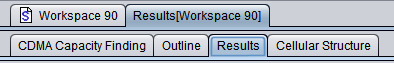
Several workspaces can be open at the same time – different workspaces are shown as tabs at the top of the user interface. The size and position of the SEAMCAT subpanel graphical user interface (GUI) is minatained when switching from one workspace to another for ease of  comparison between workspaces.

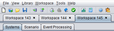Figure 20: Several workspaces in different tabs

2.3 Typical SEAMCAT workflow

When using SEAMCAT for a compatibility analysis, a typical workflow would be as follows:

1. Create or update a simulation workspace;

2. Set the simulation control parameters (number of events, debug mode or not);

3. Run a simulation;

4. Analyse the event generation results, modify the input scenario if necessary and re-run the event generation;

5. Perform one or more interference calculation runs;

6. Generate a simulation report.

 

Figure 21: Typical work flow when using SEAMCAT

 

In addition to these basic steps further ones may be useful for different purposes:

• Save workspace as an XML compliant file for later (repeated) work or for sharing with other users;

• Create or update elements in the equipment library for repeatedly used equipment types;

• Import a library;

• Use of batch job, to serialise your work;

• Share your workspace with others;

• Use of an Event Processing Plugin for advanced scenario specific calculations.

2.4 Simulation Workspace

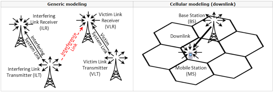
2.4.1 Scenario workspace

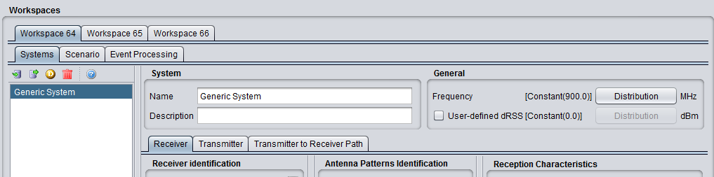
A scenario workspace can be seen as a working environment for a given study where all input fields are editable. It consists of the following three tabs:

• Systems: This allows setting the characteristic of the systems to investigate (generic Tx, Rx and path between Tx/Rx or cellular general settings, positioning);

• Scenario: This sets the simulation scenario, i.e. the selection of the systems to be used as victim or interferer(s) as well as the path between the victim and the interfer(s), the number of events and optional selection of debug mode;

• Event processing: The event processing plugin (EPP) environment allows the processing of intermediary SEAMCAT results for each simulated event. Some EPPs are available built in to the tool, but it is also possible to create customized EPPs. 

 

Figure 22: Illustration of the workspace scenario (Highest hierarchy level)

2.4.2 Results workspace

When a simulation is performed, SEAMCAT automatically generates a separate workspace to contain the results which appears as a separate tab entitled ’Results[Workspace xyz]’ and stores read only information.

Figure 23: Illustration of the workspace results (Highest hierarchy level)

 

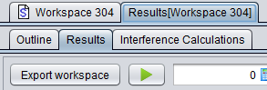
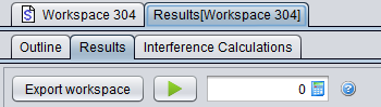
It is not possible to edit any of the input fields in the results tab. It is however possible to select ‘Export workspace’ to generate and open a new workspace scenario entitled ‘Exported Workspace xyz‘ :

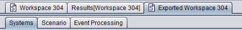
Figure 24: Illustration of exporting a results workspace into a scenario workspace

 

 The results workspace consists of the following tabs depending on the scenario set-up:

• Outline: The outline of the simulation can be seen with both a summary of the dRSS and iRSS calculation and a graphical overview of the Tx/Rx positions for the victim and interferer(s);

• Results: gives access to a list of all results generated by SEAMCAT and from the EPPs used in the simulation;

• Interference calculations: It gives access to the Interference calculation engine;

• CDMA Capacity Finding: This panel is only available when a CDMA system is used in the scenario. It indicates the non-interfered capacity (i.e. number of UEs) when the network is gradually filled up with UEs while measuring a specific system outage depending on uplink (UL) or downlink (DL) configuration;

• Cellular Structure: This panel is only available when a cellular system (CDMA or OFDMA) is used in the scenario. It shows the results of the cellular specific simulation – i.e. layout of the cells, position of users and indication of dropped users.

 

2.5 Create or update a simulation workspace

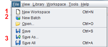
To start, create a new workspace (see 1 in Figure 25 or open an existing one (2). 

 

A simulation scenario is a part of a scenario workspace, which defines all technical parameters of modeled links as well as some related modelling assumptions, such as physical (mutual) placement of transceivers, propagation modelling settings and so on. Within SEAMCAT a simulation scenario is based upon the concept of links. A link stands for a pairing of one transmitter with one receiver[1] operating together in a given wireless system. Such a link is also called a “system link”.

When a new workspace is created, all of its scenario elements are populated with default values (representing a hypothetical interference case between two systems at 900 MHz, as shown in Figure 27). Therefore after creating a new workspace the first step should be to review and modify the scenario parameters so that the resulting simulation scenario reflects the configuration of the wireless systems to be simulated. 

To create or update a simulation workspace, the following steps need to be followed: 

1. Set the technical characterisitic of the various systems that you want to investigate. In the example of Figure 26 the first system is Generic and the second one is an OFDMA UL system. Do not forget to export the systems used to the library environment so that they can be reused  at a latter point of time. 

   
   

   

   Figure 27: Setting various systems (import/export to library environment)
   
   

    

   
   

   

   
   
   Figure 28: Overview of the various systems which can be simulated in SEAMCAT  (i.e. Generic and cellular)
   
   

    

2. Set the scenario (see section ‎10);

3. Set the path characteristics between the victim and the interferer (relative position, interferer’s density, path loss correlation and propagation model). Links can also be added, duplicated, etc...;

4. The number of events to simulate can be set in the simulation control panel. It is also possible to choose  whether to run a simulation in the debug mode or not;

5. Having reviewed the scenario, the simulation can be run.

 

 

---

[1] Cellular systems with multiple receivers (downlink) or multiple transmitters (uplink) are handled differently

2.6 Batch operation

 The SEAMCAT's Batch function allows automation of repetitive compatibility studies by scheduling several SEAMCAT simulations to be done in one run of the programme. This is done by setting up a simulation schedule with instructions on how to change certain variable scenario input parameters in several consecutive simulations. One typical example of using SEAMCAT batch functionality would be to perform multiple simulations in order to study interference probability on identical scenarios with only small frequency changes between them.

A new batch can be created directly from the quick menu button or you can open an existing batch file using the usual open icon. The following menu button can be used for the batch

 

The batch environment, as shown in Figure 28 consists of 3 panels (#1), identification, control and Workspaces.

 

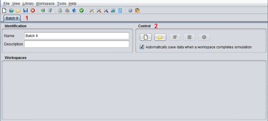
The control panel provides the following buttons dedicated to workspaces:

 

When several workspaces are opened in the batch mode environment, parameters can be directly modified in the workspace with an unlimited number of times by adding new simulations to the batch schedule until the intended variation of input parameters is fully covered by all entries. 

It is also possible to save workspace results automatically after completing their simulation. 

 

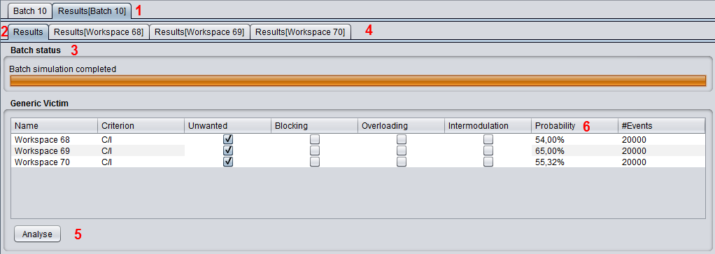
Batch results (Figure 29 #1) are available when the batch simulation is started. A result tab (#2) is by default active indicating the progress of the batch work (#3) and provides interference calculation engine capability (#5). When pressing the analyse button the ICE is activated and the probability of interference is displayed (#6).

The results vectors for each workspace are also available (#4) for scrutiny.

 

If the “debug mode” is selected and a batch is run, the batch will stop until the log window is closed.

2.7 Running and stopping a simulation

A simulation is started when clicking on the Start button in the simulation control part of the Scenario tab  (). The simulation starts and all other commands/buttons are, meanwhile, disabled except the stop button (). SEAMCAT automatically performs the consistency check of the scenario parameters before starting the event generation (see Section ‎2.9).

The simulation runs until the number of events has been performed or if the simulation is stopped prematurely by pressing the stop button. 

 

2.8 Running from the command line

 User can run SEAMCAT from Command Line which helps if you want just to run simulation and get the results. This feature is useful to run SEAMCAT simulation on number of already prepared workspaces, or if resources of the computer is an issue. In Command Line SEAMCAT just run the simulation on already prepared workspace and Graphical User Interface is not launched.  Find below some tips for using SEAMCAT in a command line environment. 

A command line launch of SEAMCAT (i.e. without GUI) is possible using the same seamcat.jar file that you have downloaded.  From the command line with a workspace file called "myWorkspace.sws" the following command will It will launch the workspace and save the results in myWorkspace.swr by default.

Several options are possible. The result file name can be changed by using the option: result=myWorkspaceResults.swr and the number of events can be specified by using the option: events=12345. The example below uses all these parameters: 

 you will see the following when setting 12 events:

If there is an issue with Java machine memory size, user can increase memory for the simulation, for e.g.

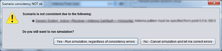
2.9 Consistency check

The consistency check function is run automatically before the start of an event in order to detect erroneous or inconsistent values in the scenario definition (see Figure 32). You can also trigger it manually as illustrated in Figure 33. The aim of the consistency check is to prevent runtime exceptions during the simulation due to incorrect input values.

 

 

The consistency check includes:

• Warnings if odd configuration are detected for random parameters, such as negative antenna height, etc;

• Consistency between inter-dependent parameters such as: C/I, C/(N+I), (N+I)/N, and I/N;

• Verification of the application range of propagation models.

 

In case it fails, the scenario consistency check will pop up a message window like the below

 

 

These warnings may be ignored in some cases, but you should be aware of the following:

• Consistency checks are generally connected to non valid values which cause runtime exceptions during the simulation

• Each runtime exception generates an appropriate error message which is recorded on the seamcat.log file (located on your SEAMCAT home directory):

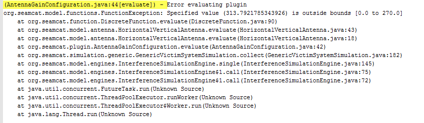
Note that the yellow marked header format can be changed as described in Annex 20.

 

 

• Logging the error messages takes time, hence it significantly increases the simulation time;

• Depending on the scenario (in particular the number of events simulated) the amount of the seamcat.log file might readily grow up to some tens of Mega Byte per simulation run.

 

It is therefore highly recommended to solve the reported issues prior to run the simulation. Further information on the meaning of consistency check and SEAMCAT error message is available in ‎ANNEX 19:.

Section ‎14.3.2 presents the implementation of the consistency check in the source code and for plugin development and its graphical results. 

 

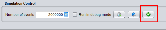
2.10 Simulation control

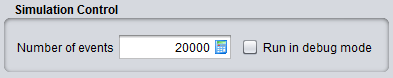
The simulation control setting “number of events” is used to determine the number of events you want to simulate. The “Debug mode” feature is described in Section ‎2.14. These control settings are accessible from the Scenario tab. 

 

2.11 Simulation results overview

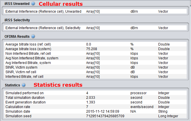
Once a simulation is complete a workspace result (see Section ‎2.4.2) is automatically created within SEAMCAT where it is possible to extract any results vector. Depending on the nature of the victim system (i.e. generic, CDMA or OFDMA), the results vectors may vary. Further details about the nature of the results can be found in Section ‎12.

The bottom of the results panel contains the scenario statistics of the simulation’s run (number of processor utilised, total simulation duration etc…). The statistics display is irrespective of the radio system simulated. 

 

2.12 Saving options in SEAMCAT

2.12.1 Saving workspace and batch

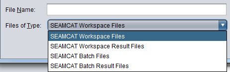
Workspaces can be saved <CTRL+S> or “save as” (either scenario or results)/batch by using the default option SEAMCAT offers in the File menu. The file extension is appended automatically. These are SEAMCAT-specific file extensions. The .sws, .swr, sbj and sbr format are equivalent to a .zip file. Table 5 provides an overview and a description of the files contained per extension.

When closing SEAMCAT without previously having saved or closed the workspace, a prompt window will appear asking whether any changes to the workspace should be saved.

 

 

 

 

2.12.2 Saving results - file extension

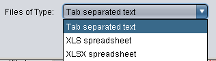
Saving workspace results will store all simulation calculations in the workspace. Vector results can also be independently saved using one of the three different file extensions: tab separated text, xls spreadsheet and xlsx spreadsheet. The various extension options are illustrated in Figure 39.

 

2.13 Simulation report

Any simulations and their results overview can be presented in a report. This report is automatically generated by SEAMCAT. Select the Report command from the Workspace menu, click on the Report icon of the toolbar () or press <CTRL+R> to activate the Report options window:

 

 

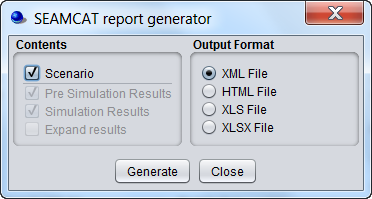
In this dialog window, the contents of the generated report can be configured, by checking or un-checking following items:

• Scenario: It indicates whether all scenario parameters should be included or not;

• Pre Simulation results: Pre-simulation is a result group where a simulation can store results that are calculated before the simulation starts. This is used primarily for the cellular simulations were complex calculations are conducted before the simulation begins (e.g. capacity findings for CDMA). For some simulation this can be empty. Currently the generic simulation has no need for presimulation results and therefore leaves the group empty;

• Simulation results: It indicates whether simulation control parameters should be included or not;

• Expand results: It allows expanding tabular data by checking or unchecking the Expand tabular data option.

There are three formats for the report: 

• XML File (default);

• HTML File;

• Excel File (.xls and .xlsx).

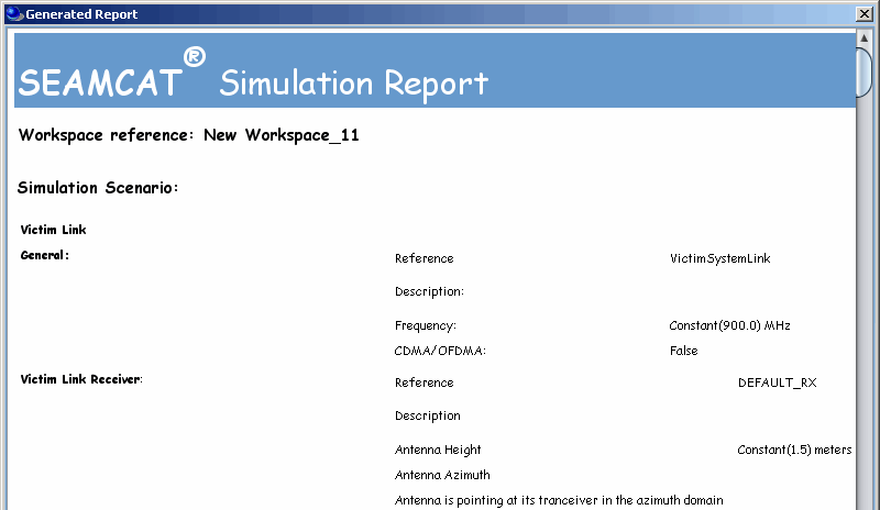
When clicking on “Generate”, a file is automatically generated in the “reports” folder under the SEAMCAT home directory (see Figure 15).

For all other data types the output is similar to their display in the workspace tree view except that couples of values defining user-defined random data, functions, and radiation patterns are fully expanded. 

 

 

2.14 Logging function for debugging

SEAMCAT allows two options to generate two distinct log files. An automatic SEAMCAT log that monitors the behaviour of the application, and a user debug log to check how the computation is performed.

seamcat.log: This log file is automatically generated by SEAMCAT and is intended to be used to debug the Java application mainly in case of a crash of the application or when an exception in the code occurs. You can select/browse the filename and directory from the SEAMCAT options and also the log level.

Figure 42: SEAMCAT configuration

 

Figure 43: Seamcat.log log file automatically generated by SEAMCAT

 

Debug Mode: Running a simulation in “debug mode” Figure 44 is used for detailed check of the simulation process. Selecting this option, SEAMCAT will generate a log file where all interim results of simulations including what random values were generated for parameters defined as functions or distributions. This information is very useful for further inspection. The log file will be automatically stored in the sub-directory "Logfiles" of the main SEAMCAT directory. The debug option reduces the number of events to 5 events for the sake of limiting the size of log file. The generated log file may be reviewed using standard reading tools, such as Notepad, MS Windows, etc. 

 

Figure 44: Selection of the debug mode

 

The output of the file (filename_date_number.log) is indicated at the bottom’s right corner of the SEAMCAT application window (see Figure 45) as well as in the first line of the log display as shown in Figure 106.

 

Figure 45: Filename and directory output for the debug log file

 

 

An example fragment of such a debug mode log file is shown in Figure 46. The settings for generating the log file in the SEAMCAT configuration panel can be modified as described in ANNEX 20:.

Figure 46: Example of a debug mode log file

2.15 Play / Replay an event

In the Results tab, there is access to a list of all the results from SEAMCAT and from the EPPs used in the simulation giving the option to “Play/replay” one event, and a log of the calculation will be made available.

When inspecting the dRSS or iRSS vector, an event may be identified and further investigated by using the replay feature. For that, identify the event number to replay, insert this number and click on the ”play” button . A new tab called <Replay [event = x]> will be created and will contain an “Event Result” panel on the left and a “Log Trace” on the right hand side. This log file is automatically saved under the “logfiles” folder in your home directory.

Figure 47: Illustration of the play/replay feature

 

Figure 48: Illustration of the Replay tab with “Event Result” on the left and “Log Trace” on the right

 

Doing cellular system simulation the play/replay function allows re-runnning a specific event and redisplaying a cellular structure layout as shown in Figure 49. Inspecting an event allows the validation of the configuration of the simulated workspace.

Figure 49: Example of the play/replay feature for a cellular network

 

2.16 Testing propagation models

A sanity check on the suitability of a propagation model can be done by clicking on <Tools/Test Propagation Models> in the main menu of SEAMCAT, by clicking on the icon () of the toolbar or by pressing <CTRL+SHIFT+M>. With this feature, it is possible to evaluate the result while using a certain propagation model.

 

Figure 50: Access to testing propagation model

 

For that, choose the propagation models to compare them. It is possible to compare 2 or more propagation models with this interface.

Figure 51 shows that the SEAMCAT resulting attenuation from the free space is 101.47 dB where the free space path loss is defined as:

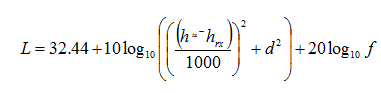        (Eq. 16)

where d is given in km and f is given in MHz. This results in

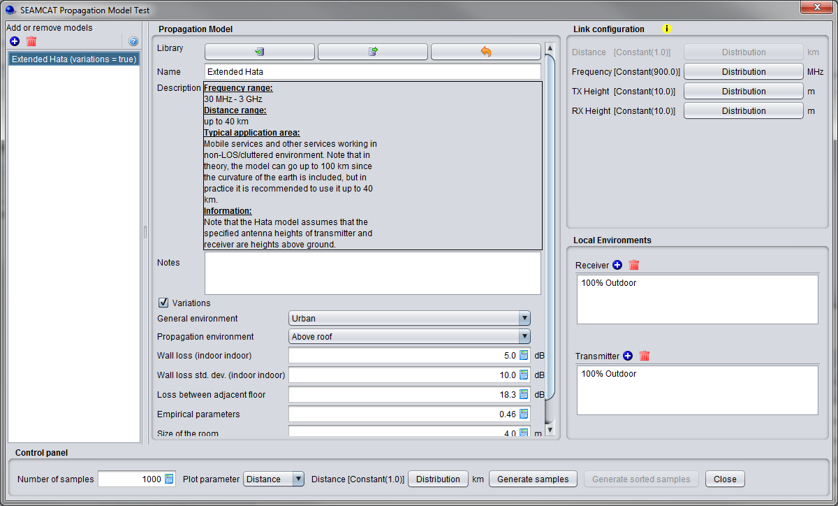
Figure 51: Illustration on to check the propagation model results

 

If one parameter is chosen as a distribution (for instance distance), then the button <generate sorted samples > is activated. Pressing it enables you to plot your results according to a sorted X-axis from min to max.

Finally click on <Generate samples> or <generate sorted samples> (depending which one is active) to view the results. If no results are displayed, check the Java console for any error messages.

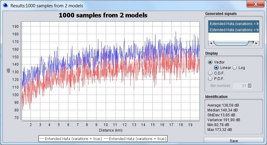
Figure 52: Example comparing 2 propagation loss using the “generate sorted samples”. You can display the vector in linear or logarithmic scale 

2.17 Testing distribution functions

A sanity check on distributions can be done with the test distribution function from the menu bar of SEAMCAT. The result of generating random values using a particular distribution type can be tested by selecting the <Test Distributions> command from the Workspace menu, by clicking on the icon of the toolbar () or by pressing <CTRL+SHIFT+D>. This could be e.g. used to analyse the statistical qualities of generated random variables. 

Figure 53: Access to testing unwanted emission function

 

Figure 54: Illustration of the distribution check routine

 

2.18 Testing unwanted emissions function

A sanity check on the unwanted emission calculation can be done by using the <Test Rel. Unwanted> emission function in the menu bar of SEAMCAT, by clicking on the icon of the toolbar ( ) or by pressing <CTRL+SHIFT+U>. The definition of unwanted emissions mask can be checked by calculating the actual unwanted emissions for given mask in a given VLR bandwidth applying a certain ILT-VLR frequency offset:

 

 Figure 55: Access to testing unwanted emission function

 

This feature allows to directly extract the unwanted emission by entering the frequency separation, the receiver bandwidth and the spectrum mask as shown in Figure 56. 

Figure 56: Illustration of the unwanted emission function check routine

 

2.19 Multiple vectors comparison

All the vectors (or a subset) that have been generated for one workspace or more can be seen at once. For this, the <Compare Vectors> command is available by clicking this icon  or by pressing <CTRL+SHIFT+V> to open the dialog box in Figure 57.

 

• It allows displaying multiple vectors that are resulting from the simulations (batch or not);

• It allows adding external vectors from a past simulation;

• It allows changing the text of the legend by double clicking on the vector.

Figure 57: Illustration of the compare vectors feature

2.20 Pocket calculator

SEAMCAT contains a builtin pocket calculator. Select the command < Tool/Pocket Calculator> from the Workspace menu, click on the pocket calculator icon of the toolbar ( ) or CTRL+SHIFT+C to activate the Pocket calculator window: 

 

Figure 58: SEAMCAT pocket calculator

 

The calculator can also be accessed from the graphical user interface when a scalar is to be entered as shown in the example of Figure 59 with the wall loss attenuation of the Extended Hata propagation model.

Figure 59: Access to the calculator from the GUI panel

2.21 Online manual and help content

SEAMCAT provides a direct access to the online manual by clicking on the following symbol .  Each panel contains a specific link where detailed information on the feature or algorithm can be found. In case of need for further information, clarification, or in order to supply additional information or improvements to the manual that could be useful for other users of SEAMCAT, please contact the ECO project manager at seamcat@eco.cept.org

2.22 Report enhancements and bugs

The SEAMCAT tool is thoroughly tested but in case of need to report bugs or enhancements, send an email to seamcat@eco.cept.org by describing the issue and attach relevant files (i.e. workspace files, screen shots, system log file etc…). Further information on the log file can be found in section 2.14.

It is advised to use the STG template for this, which can be downloaded by clicking on the “bug report” button: 

Figure 60: Bug report

2.23 Installing plugins in SEAMCAT

From the SEAMCAT library menu it is possible to install a library as a .jar file. By creating a new .jar entry and adding the file SEAMCAT will now include this plugin to be selectable when configuring scenarios. 

Figure 61: Installing plugins

After installation the installed plugin can be seen in the SEAMCAT library. Any plugins can be loaded from this interface (e.g. Propagation Model Plugin, Event Processing Plugin, coverage radius etc…). Further description on the library is available in section ‎13.

Figure 62: Library jar installer

2.24 Pausing and RESUMING a simulation

A simulation can be paused when clicking on the Pause button in the simulation control part of the Scenario tab ( ). The simulation pauses and all other commands/buttons are, meanwhile, disabled except the stop button (  ). The simulation is resumed by clicking on the Resume button (  ).

Figure 63: Simulation control inside the Outline window in the Results tab during run time

 

2.25 Considering time domain Tx activity

Methods for applying time-domain activity of transmissions in SEAMCAT simulation

1. Tx power Distribution

• Applicability: cellular or generic systems with multiple interferers where individual transmitters exhibit independent random time domain behaviour (e.g. mobile networks, SRDs)

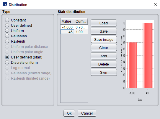
The user can set User defined (Stair) distribution where for the active state the actual power of transmitter is simulated, and for the non -active state set an arbitrarily low Tx power (e.g. -1000 dBm) is assumed, effectively simulating an “off” transmitter.

In the System settings under Transmitter / Power, the user needs to select Distribution, select User defined (stair) and input a cdf function. This is particularly useful for cases where a scenario needs to simulate on and off periods such as with Duty cycle or similar. For example, if a Tx is working with 46 dBm power which is transmitted for 30 % of time the settings would need to be as shown in the figure below.

In simulation, at each trial the Tx power will be generated with 30% probability to be 46 dBm. Please note that in this case 70% of events will be non-interfered from this transmitter and depending on the scenario, the number of events might need to be adjusted to obtain a sufficient number of relevant interfering cases.

2. Setting Uniform (and Closest interferer) mode of simulation together with Transmitter density and Traffic

• Applicability: Generic systems with multiple interferers of a specific density and random positioning, where individual transmitters exhibit independent random time domain behaviour (e.g. SRD)

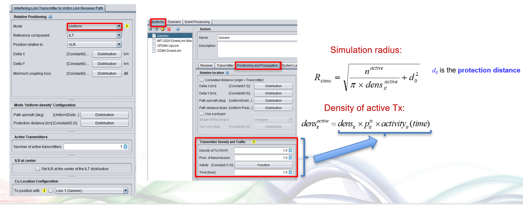
In Systems under Positioning and Propagation, the user can set Transmitter Density and Traffic parameters. This panel defines the parameters Transmitter density, Probability of transmission Activity and Time. With these parameters SEAMCAT calculates the density of active transmitters to simulate. To use these settings in the Scenario, the user needs to select Uniform mode and adjust the number of active transmitters and the protection distance (if relevant according to the scenario).

The system then calculates an appropriate simulation radius so that the specified density of active Tx is fulfilled with the entered number of Active transmitters. In this case only transmitters which are active are simulated in the event and considered in calculation of Interference vectors. These settings are particularly useful when the transmitter density is known, as it is the case for many SRD devices.

The Closest interferer mode is similar, but it generates only one active transmitter which is closest to the victim under the given settings.

 

3. Adjusting Tx power to averaged power instead to actual power when working

• Applicability: Generic or cellular systems with a high number of interfering transmitters and a large separation distance to the victim receiver (e.g. satellite space station receiver)

In some cases, the user is interested in the averaging effect of interference from a high number of Tx, so the effect of a proportion of Tx working with max power part of the time would be equivalent to all Tx working with average power all the time. In that way maximal power of the transmitter could be averaged.

For example, if we have a transmitter with an average transmit power, P= 15 dBm with an activity factor of 0.02, the average power can be calculated as:

• an average power to be used for each active user:

P_a = 15 + 10log₁₀(0.02) = –2 dBm.

This power can be set under System settings / Transmitter / Power settings of the Transmitter. An example of this usage for mobile terminals in cellular systems can be found in section 2.2.3.7 of Report ITU-R M.2241 and in Report ITU-R M.2292-0.

 

4. Conditional probability formula & law of total probability

• Applicability: Scenarios with a single interferer with time-dependent transmission, or multiple time-synchronised transmitters (e.g. TDD cellular networks)

In some cases, it is appropriate to use a conditional probability formula to post-process the SEAMCAT probability results. In this case the SEAMCAT simulation is run with max power and a fully loaded system, and the resulting probability is combined with a conditional probability to calculate the probability of interference according to the Law of total probability.

For example if it is assumed that Tx is active 30% of time then the total probability of interference can be calculated as:

P(Interf) = P(Interf /Active)*P(Active)+P(Interf/non_active)*P(non_active)

P(Interf) = P(interf /Active)*0.3 + P(interf/non_active)*0.7 = P(interf /Active)*0.3 + 0

In this method it is assumed that the proportion of time when the Tx is not active is equivalent to adding an equivalent proportion of additional non-interfered events into the simulation. This approach has the benefit of not using additional computational resources to simulate events for which probability of interference is zero, and instead account for these cases by simple post-processing.

This approach can also be extended to combine results of TDD cellular network interference from separate simulations of downlink (DL) and uplink (UL) according to:

 

where:

is the total interference probability

 are the individual results of probability of interference from DL and UL respectively, calculated in separate workspaces

 are the DL and uplink TDD ratios

 

For example, for a typical case of a TDD DL/UL split of 75%/25%:

 

 

5. Separate activity vector combined with extracted results vectors

• Applicability: where detailed event level results are needed, or post-processing of cellular capacity results taking into account time-dependent activity (e.g. cellular victim systems with time-dependent interferers)

In some cases, it is necessary to extract vectors of wanted (dRSS) and interfering signals (iRSS), or other results such as cellular capacity, for post-processing. These vectors can be extracted and combined with time-dependent activity as follow:

• Create SEAMCAT workspace and run simulation assuming full power and fully loaded systems

• Export desired vectors for VSL and all ISL

• In external software, generate a random activity function which results in 1 with probability according to the specified activity factor and 0 otherwise; produce as many vectors as needed of this function.

• Multiply the relevant signal vector from SEAMCAT with the activity vector (note that iRSS_unwanted and iRSS_blocking coming from same interferer needs to be multiplied with the same activity vector)

• Use these multiplied vectors for calculation of interference or further post-processing as needed.

 

6. Reduce the number of active Tx to simulate

• Applicability: allow to reduce computation time by reducing the number of active Tx to simulate.

For a fixed simulation radius and a fixed density of Tx, assuming a certain duty cycle of x% for instance means that x% of the Tx interferer is “ON” (i.e. active) and “OFF” the rest of the time. So for that simulation radius, and fixed density, it is not needed to simulate the Tx that are “OFF”. This is similar to the option 1 “Tx power Distribution”, but faster. Simulating x% of Tx that are active (at full power) reduces computation time.

• For fixed simulation radius and fixed density of interfering transmitter, calculate the number of total interfering transmitter. Apply the duty cycle ratio to calculate the number of active transmitters.

• In SEAMCAT workspace, select the mode “none” (or “standard” in new version), set the “simulation radius” and set the “number of active transmitters”.

 

1. Additional Loss Distribution

• Applicability: cellular or generic systems with multiple interferers where individual transmitters exhibit independent random time domain behaviour (e.g. mobile networks, SRDs)

Another solution without the need for normalise and could work with Power lock / unlock distribution is to take activity into Additional loss. It can be set at terminal level and is embedded in calculation or received level (either dRSS or iRSS) whatever is needed. I tested – it works like that.

Settings:

• Power – applying distribution with power distribution requested (if needs locking in time elements – possible to do that)

• Have Additional loss as distribution = 1000 dB – 80% and 0 dB – 20 % (this will add 1000 dB of loss to the link in 80% of time – i.e. like this terminal is not active)