12 Results
- 12.1 Scenario outline
- 12.1.1 Simulation Summary
- 12.1.2 Simulation status
- 12.1.3 Generic system outline
- 12.1.4 Cellular system outline
- 12.2 Overview of output results
- 12.3 Generic model Results
- Introduction
- 12.3.1 Generated signals results
- 12.3.2 Calculated radius
- 12.3.3 Intermodulation results
- 12.3.4 Overloading results
- 12.4 Spectrum sensing results
- Introduction
- 12.4.1 sRSS vector
- 12.4.2 WSD frequency
- 12.4.3 WSD e.i.r.p.
- 12.4.4 Victim frequency vector
- 12.4.5 Average e.i.r.p. per frequency
- 12.4.6 Average active WSDs per frequency vector
- 12.5 CDMA output results
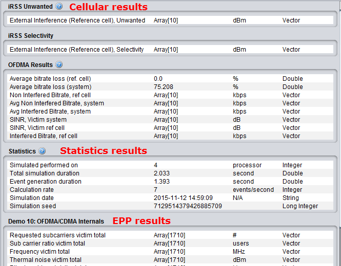
- 12.6 OFDMA output results
- 12.7 EPP results
- 12.8 Cellular Structure
- 12.9 Interference calculations
12.1 Scenario outline
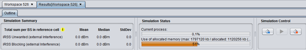
12.1.1 Simulation Summary
The simulation summary (left of Figure 242) provides a quick access to the mean, median and standard deviation of the dRSS, iRSS unwanted and iRSSblocking
The mean is computed using the simulated results in dB. The median is computed using the simulated results converted to linear values and then converted again to dB. The standard deviation (StdDev) is computed using the simulated results in dB. This is further explained in Annex A1.5.1.
12.1.2 Simulation status
The progress bar (right of Figure 242) reflects the percentage of events simulated with respect to overall number of events specified in the simulation control window in the scenario tab.
12.1.3 Generic system outline
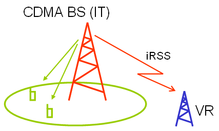
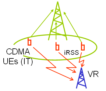
During the event generation all involved transceivers (ILT, ILR, VLR and VLT) are plotted in graphical display window placed on the simulation outline tab.
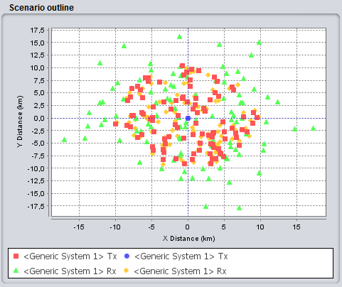
The dRSS and the iRSS vectors are shown for 100 events maximum to avoid overloading the memory and to speed the computation time. The iRSS is shown as a summation of all the interferers.
12.1.4 Cellular system outline
Once SEAMCAT has determined the number of UEs per cell either through simulation of optimal capacity (see Figure 197 for UL and Figure 198 for DL or by a value that you specify the actual simulation of snapshots begins. As with all scenarios this causes SEAMCAT to show the scenario outline (Figure 245 for UL and Figure 246 for DL).
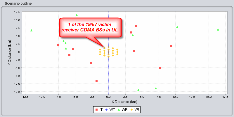
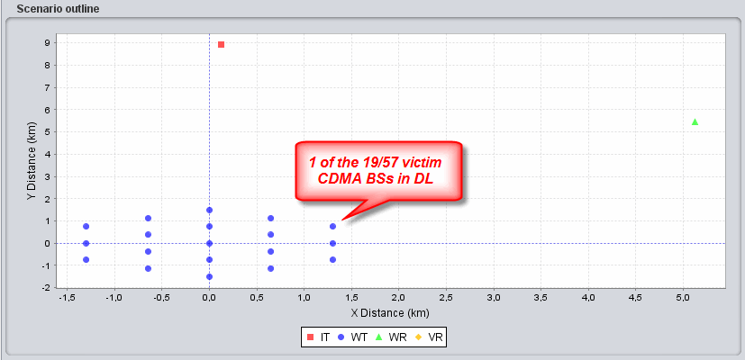
Only CDMA base-stations will appear in the Scenario outline graph. Dependent on the scenario the base-stations positioning will appear as shown in Table 50.
|
Scenario configuration |
BS role |
UE role |
Positioning |
Illustration |
|
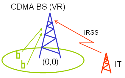
CDMA Downlink is victim |
Victim link transmitter |
Victim link receiver |
Reference cell is positioned in (0,0) |
|
|
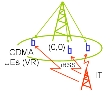
CDMA Uplink is victim |
Victim link receiver |
Victim link transmitter |
Reference cell is positioned in (0,0) |
|
|
CDMA Downlink is interferer |
Interefering link transmitter |
Interfering link receiver |
Relative to victim and reference cell |
|
|
CDMA Uplink is interferer |
Interfering link receiver |
Interefering link transmitter |
Relative to victim and reference cell |
|
12.2 Overview of output results
|
Victim system |
Intereference criteria |
|
Generic module (i.e. non CDMA/OFDMA) |
Probability of interference based on C/I, C/(I+N), (N+I)/N, I/N |
|
CDMA |
Capacity loss (i.e. number of voice users being dropped) |
|
OFDMA |
Bitrate loss (i.e. number of bit rate lost compared to a non interfered victim network) |
12.3 Generic model Results
Introduction
After running a simulation with generic system, each of these signals is displayed with indicated array size (i.e. the number of valid generated events), unit and then the type (vector, double etc..).
Double-clicking on one of the vectors, the signal dialog window (see Annex A1.5) will plot the signal as well as its statistical features.

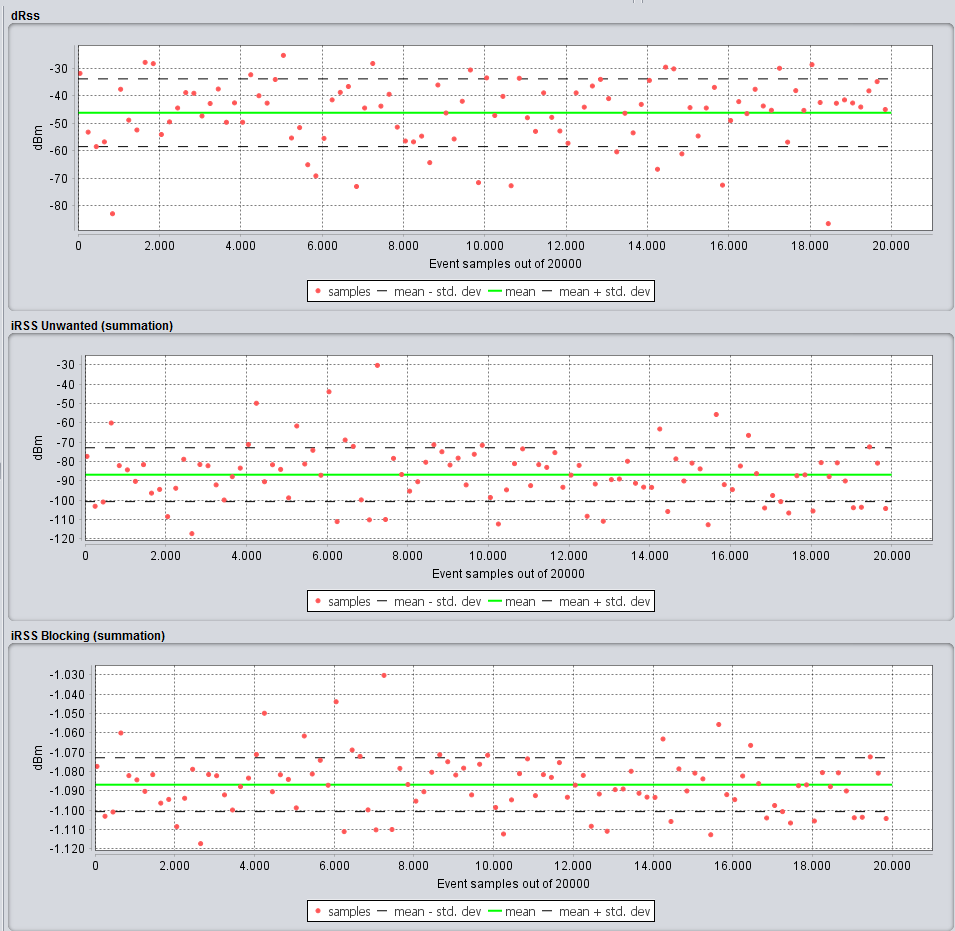
12.3.1 Generated signals results
-
dRSS folder (ANNEX 4:) with dRSS vector;
-
iRSS unwanted folder (ANNEX 5:) with as many iRSSunwanted vector for each interfering link and one vector for the sum;
-
iRSS blocking folder (ANNEX 5:) with as many iRSSblocking vector for each interfering link and one vector for the sum.
12.3.2 Calculated radius
The calculated radius folder contains the values of the coverage and/or simulation radii calculated for the event generation when set to non-correlated (See ANNEX 13:).
12.3.3 Intermodulation results
iRSS intermodulation folder (Figure 248) with as many iRSSintermod vector for each combinatory couple in case there are more than one interfering link and one vector for the sum.
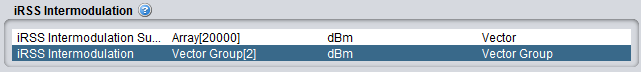
Figure 248: Intermodulation results folder
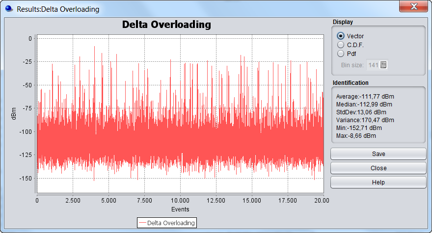
12.3.4 Overloading results
As a result of the equation described in Annex A5.4, for each event and at each frequency, the sum of the iRSSoverloading (iRSSsum_overloading) will be compared to the overloading treshold Oth(fi) at that frequency (fi). The difference, delta (in dB), will be stored.
-
When delta ≥ 0, then the receiver is overloaded at that fi (i.e. the rest of the frequency do not matter);
-
When delta < 0, then the receiver is not overloaded at fi.
If only one frequency is present, the iRSSsum_overloading is compared to the Oth(fi)and the difference will be stored for that event. If more than one frequency is present, the highest delta value will be indicated in the vector (i.e. irrespective of the frequency) such that
for each event j (where dRSS > sensitivity){
for Frequency = i to number of total frequencies{ delta_max(j) = max(delta(fi)); } (Eq. 67)
}

The output delta overloading vector is of the dimension delta x number of events
12.4 Spectrum sensing results
Introduction
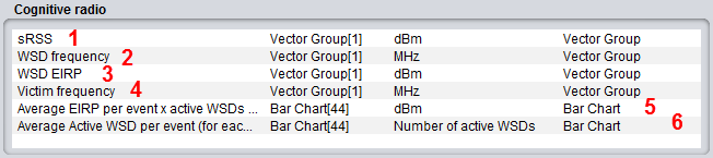
When the cognitive radio mode is activated, SEAMCAT resturns the output vector shown in Figure 251 and described in Table 52.
|
# |
Item |
Description |
|
1 |
sRSS |
sRSS value calculated at the selected WSD frequency (i.e. where the WSD is allowed to transmit) for each of the event |
|
2 |
WSD frequency |
The actual selected frequency at which the WSDs are allowed to transmit as the result of the spectrum sensing algorithm |
|
3 |
WSD e.i.r.p. |
The actual selected e.i.r.p. at which the WSDs are allowed to transmit as the result of the spectrum sensing algorithm |
|
4 |
Victim frequency |
frequency at which the victim device transmits per event |
|
5 |
Average e.i.r.p. per event x active WSDs (for each frequency) |
average e.i.r.p. per event for all the active WSDs transmitting at a certain frequency |
|
6 |
Average Active WSD per event (for each frequency) |
|
At the end of the simulation, SEAMCAT provides a set of output vectors as above. Then you can perform the interference probability calculation as previously described.
12.4.1 sRSS vector
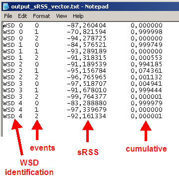
The sRSS vector (dBm) is merely the sRSS value calculated at the selected WSD frequency (i.e. where the WSD is allowed to transmit) for each of the event. Figure 252 displays the vector for each WSD. You can select any or all of the WSD (#1). The same applies to the CDF and density graphs (#2).
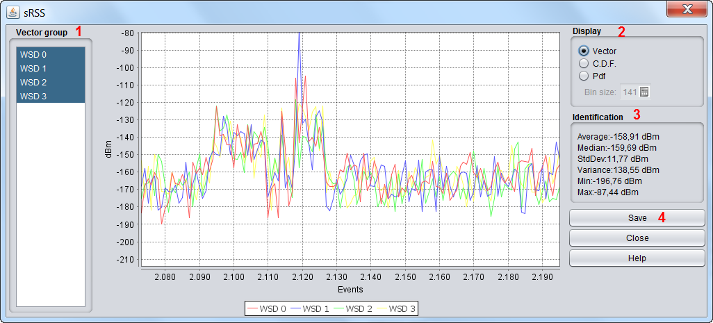
You are able to save the results (#4) as .txt file for further post-processing.
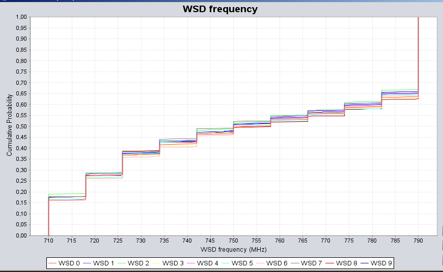
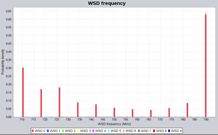
12.4.2 WSD frequency
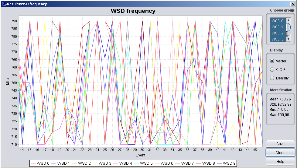
This vector represents the actual selected frequency (MHz) at which the WSDs are allowed to transmit as the result of the spectrum sensing algorithm.
|
|
|
|---|---|
|
(a) |
(b) |
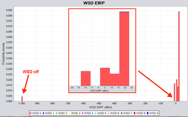
12.4.3 WSD e.i.r.p.
The actual selected e.i.r.p. (dBm) at which the WSDs are allowed to transmit as the result of the spectrum sensing algorithm. This vector displays the e.i.r.p. for each of the WSD for all the events. In the example presented in Figure 256, the WSDs are transmitting with a e.i.r.p. between -10 and 20 dBm and -1000 dBm (equivalent to WSD switch off).
12.4.4 Victim frequency vector
The victim frequency vector (MHz) represents the frequency at which the victim device transmits per event.
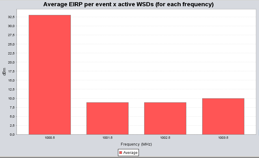
12.4.5 Average e.i.r.p. per frequency
It presents the average e.i.r.p. per event (dBm vs MHz) for all the active WSDs transmitting at a certain frequency such that:
 (Eq. 68)
Let us assume a different example from above, where 4 channels have been identified for the WSD to operate. Figure 257 shows that on average 33 dBm, for one event, was transmitted by the active WSDs at 1000.5 MHz , 8.82 dBm at 1001.5 MHz etc...
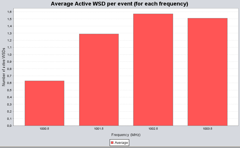
12.4.6 Average active WSDs per frequency vector
It provides the average number of active WSD per event for a specific frequency:
 (Eq. 69)
Re-using the example of Figure 257, Figure 258 indicates that, with for instance 5 WSDs set as input parameters, an average of 0.63 WSDs were active at 1000.5 MHz (with 33 dBm e.i.r.p. Figure 257), 1.29 WSDs were active at 1001.5 MHz (with 8.82 dBm e.i.r.p. Figure 257), 1.57 active WSDs at 1002.5 MHz and 1.51 active WSDs at 1003.5 MHz. It can also be noted that in this particular example, the sum of the active WSDs across the selected frequencies is 5, meaning that all the simulated WSDs have been active and none have been turn off.
12.5 CDMA output results
12.5.1 CDMA capacity finding
During the pre-simulation part, the system estimates the load of the network as shown in Figure 259. The results are presented as in Figure 260.


12.5.2 CDMA results
Once SEAMCAT has completed the simulation, the results are shown as displayed in Figure 261, when the CDMA network is the victim. This figure presents the difference between the 2 steps power balancing process (1-initial power balancing, 2- power balancing after introduction of an external interference), that is to say " non-interfered capacity " is the number of UEs in the victim network prior to adding an external interferer and "interfered capacity" is the number of UE in the victim network after adding the external interference.
-
Units: number of connected UEs;
-
Initial capacity: Number of connected UEs before any external interference is considered;
-
Interfered capacity: Results after External interference is applied;
-
Excess outage, users: How many UEs were dropped due to external interference;
-
Outage percentage: Percentage of UEs dropped due to external interference.
When the CDMA system is the interfering link, the total received power at the receiver in the victim link, due to the transmit power of all the active mobile stations in the three cells of the center cell site of the CDMA cluster, adjusted for spectral masks, etc., is counted as the interfering power in the victim link. Therefore, it is not necessary to keep track of any capacity loss in this case, unless the victim link is also a CDMA system.


SEAMCAT is able to calculate (for CDMA) 3 losses:
1) Loss of UEs for the whole network based on the before and after number of UE
System capacity loss = 100 - (interfered_capacity/ non-interfered_capacity)*100 (Eq. 70)
2) Loss of UEs for the reference cell based on the before and after number of UE
Ref cell capacity loss = 100 - (interfered_capacity/ non-interfered_capacity)*100 (Eq. 71)
3) Loss of UEs for the whole network based on the total number of dropped UE
System capacity loss = total_dropped_UE_system/total_simulated_UE*100 (Eq. 72)
It is quite important to understand that there is not a 1-to-1 map between non-interfered active/interfered users and the dropped users. Dropped user can occurs at many level of the algorithm, it can be due to:
-
“Unable to connect during first initialisation of UE” during the initialization (long before the step 2 balancing) but still it will be registered;
-
During the balancing. For CDMA UL (no cell selection activated), when the noise rise is balanced, i.e. the number of UE is acceptable is reached after introduction of external interferers, then the BS estimates the signal-to-interference ratio (C/I), measured in bit energy-to-noise density ratio Eb/N0, and compares it to a target value (Eb/N0_target). If the difference between the estimated C/I and the Eb/N0_target, is higher than a call drop threshold, then the UE is dropped;
-
“Eb/No requirement does not meet while scaling the channel power” during the scaling power.
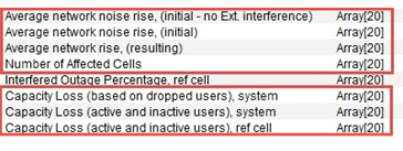
12.5.3 CDMA results for cell selection algorithm
When the CDMA “cell selection” algorithm is simulated, the following output vectors are also available for scrutiny:
-
Average network noise rise (initial without external interference): value at step 1 (i.e. before the algorithm - see Annex A15.3.2)
-
Average network noise rise (initial): value at step 5 (i.e. before the algorithm - see Annex A15.3.2)
-
Average network noise rise (resulting): value at step 10 (i.e. after the algorithm - see Annex A15.3.2)
-
Capacity loss in the whole network (for each event, calculate the capacity loss in %).
-
Capacity loss in the reference cell per event
-
Capacity loss in the worst cell per event (the first strongest cell: selectedCell[1]). The cell-ID can be different from event to event but the capacity loss is to be extracted).
-
The number of cells affected per event.
12.6 OFDMA output results
The results of the OFDMA simulation are given in terms throughput loss of the OFDMA victim. Figure 263 presents an overview of the simulation results. It consists of the achieved bitrate (with or without external interference) for the reference cell or the whole system.
A summary of the bit rate loss expressed in percentage for both the reference cell and the entire OFDMA network (i.e. the whole system) is also available. The percentage calculation is performed for each snapshot and the mean of the percentage over all the snaphsots is deduced.


12.7 EPP results
In case an EPP is used and it returns a set of result, they will also be included next to the statistic panel as shown in Figure 264. The EPP can also produce results like Single values, Vectors, Vector groups, Scatter diagrams, Barcharts.
12.8 Cellular Structure
Introduction
When simulating CDMA or OFDMA systems, you will have access to the additional tab "Cellular structure", which will become active after completion of the simulation. This new tab allows you to inspect the internal details of CDMA/OFDMA cluster based on data on one event.
After a simulation these GUI parts are used to provide access to calculated results but also detailed insight into the last event of the simulation as illustrated in Figure 265, but you can reproduce any event using the play/replay feature (Section 2.15).
The “Summary of event #n” and “inspect selected element” panel of Figure 265 are shared components from the CDMA and OFDMA module.

12.8.1 Plot configuration
The top part of the detailed system information screen contains a range of checkboxes used to control which information is plotted (Figure 266). A full description of each checkbox is given in Table 53.

|
Name |
Description |
|
Users |
Plot active UEs across the entire system |
|
Dropped users |
Plot dropped UEs across the entire system |
|
Connection lines |
Plot active connections for all active UEs – this only shows if “UEs” are checked |
|
TX stats |
If system is downlink this toggles the display of the transmit power of each base-station. If system is uplink this toggles the display of the noise rise of each base-station as well as the total interference experienced by that base-station. Also the number of active UEs connected to each base-station is shown – regardless of link direction. |
|
Antenna Pattern |
Toggles a visual representation of the antenna pattern of the selected base-station. This is mostly interesting in tri-sector scenarios. The plot of the antenna pattern can be used to ensure that the correct sector is selected. |
|
Cell centre |
Toggles the display of base-station position within the cell. |
|
External Interferers |
Toggles the display of external interferers. This only has effect when CDMA is victim. |
|
Cell ID# |
Toggles the display of the internal SEAMCAT cell id next to the cell centre |
|
Legend |
Toggles the display of the legend in the top left part of the main plot area |
The main part of the CDMA network Details window is used by the main plot. The plot shows a visual representation of the last snapshot and should be used to validate that the input parameters actually corresponds to the system that should be simulated. The plot allows for heavy user interaction. A very basic example is shown Figure 267 below.
 Figure 267: Main plot of CDMA network
12.8.2 Summary of event #n
The “Summary of event#n” panel provide a few metrics on the number of users simulated Figure 268
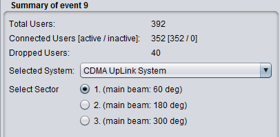
Table 54: Snapshot summary description
|
Name |
Description |
|
Total Users |
The total number of UEs in the system (number of BS x UEs per cell) for CDMA (active and dropped) and number of active users for OFDMA. |
|
Connected Users (active/ inactive) |
Number of UEs connected. In CDMA and OFDMA it is assumed that all users are active. |
|
Dropped Users |
Number of Ues dropped after power balancing. If CDMA is victim it is the number of Ues dropped after introduction of interference. Note that uplink CDMA drops Ues based on the average noise rise in the system – so it is possible for a single interferer to “shut-down” the entire system (causing all Ues to be dropped). In OFDMA, the purpose is to look at the bitrate/throughput loss and not to look at the number of dropped users, but it is possible to drop users depending on the input set-up. |
|
Selected system |
If more than one CDMA network is available in the scenario, a dropdown is used to select the system. You can choose to visualise either the victim or the interfering system which has been simulated. When you select the victim system, it is also possible to see the position of the interferer. |
|
Selected sector |
When tri-sector layout is used, it allows you to see the antenna pattern for the selected sector. Note that the antenna pattern should also be selected in the plot configuration (for visualisation purpose only). |
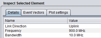
12.8.3 Inspect selected element
12.8.3.1 Detail
When an element of the main plot is selected, its detailed information is shown in a table. Further detailed are presented in Annex A15.1 with respect to CDMA network, Detailed of voice users, cell.
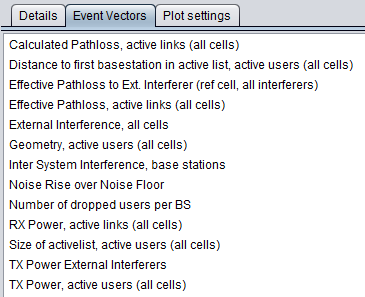
12.8.3.2 Event Vectors
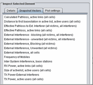
You are able to investigate some intermediary output vectors resulting from the cellular simulation.
For the position information (x,y) of the active UE details, all coordinates are always shown in the SEAMCAT coordinate system which by definition either the VLT or the victim reference cell in (0,0). Therefore, the position of the elements of an interfering CDMA or OFDMA system is based on the victim reference cell and not its "internal" reference cell.
|
|
|
|---|
|
Name |
Description |
|
Calculated pathloss |
Raw parthloss for all the active links (i.e. active UE to ist serving BS) |
|
Distance to first BS |
Distance from UE to its serving BS (first refer to cases where tri-sector is active) |
|
Effective Pathloss to Ext. interferer (all victims, all interefers) |
Effective pathloss between all the victims and all the external interferers |
|
Effective pathloss, active links |
Effective pathloss between all the victims and there respective serving BSs. Results of the below equation for all the active links |
|
External interference, all cells |
Sum of the iRSSblocking and iRSSunwanted at each victim cell |
|
Geometry |
Evaluate the Geometry for the active users for the all network |
|
Inter System Interference |
Evaluate the interference from your own network |
|
Noise rise over the noise floor |
Evaluate the Noise rise over the noise floor |
|
Number of dropped users per BS |
Evaluate the Number of dropped users per BS |
|
Rx power, active links |
Received power at the victim serving BS (UL) or active UE (DL) from its own system (used for investigating the inter-system interference from other cells) |
|
Size of active list |
Size of active list |
|
Tx power external interferers |
Tx power from the interferer |
|
Tx power, active users |
Tx power from its own system |
|
Name |
Description |
|
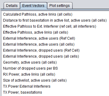
External interference, active users (all cells) |
Evaluate the external interference on all the active users for the whole network |
|
External interference, active users (ref cell) |
Evaluate the external interference on all the active users for the reference cell only |
|
External interference, dropped users (all cells) |
Evaluate the external interference on all the dropped users for the whole network |
|
External interference, dropped users (ref cell) |
Evaluate the external interference on all the dropped users for the reference cell only |
|
|
|
|---|---|
|
(a) |
(b) |
|
Name |
Description |
|
Calculated pathloss |
Raw parthloss for all the active links (i.e. active UE to ist serving BS) |
|
Distance to first BS |
Distance from UE to its serving BS (first refer to cases where tri-sector is active) |
|
Effective Pathloss to Ext. interferer |
Effective pathloss between all the victims and all the external interferers |
|
Effective pathloss, active links |
Effective pathloss between all the victims and there respective serving BSs. Results of the below equation for all the active links |
|
External interference –blocking (all victims – all interferers) |
iRSSblocking for each of the victim UE interferered by each interferer |
|
External interference –unwanted (all victims – all interferers) |
iRSSunwanted for each of the victim UE interferered by each interferer |
|
External interference –blocking (all victims) |
Aggregate external interference iRSSblocking for each of the victim UE. Sum over all the interferers |
|
External interference –unwanted (all victims) |
Aggregate external interference iRSSunwanted for each of the victim UE. Sum over all the interferers |
|
External interference, all cells |
Sum of the iRSSblocking and iRSSunwanted at each victim cell |
|
Frequency mobiles |
Vector of the frequency of the UE (in UL) for each active link |
|
Inter System Interference |
Evaluate the interference from your own network |
|
Rx power, active links |
Received power at the victim serving BS (UL) or active UE (DL) from its own system (used for investigating the inter-system interference from other cells) |
|
Size of active list |
Size of active list |
|
Tx power external interferers |
Tx power from the interferer |
|
Tx power, active users |
Tx power from its own system |
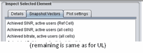
Table 60: Output vector results for OFDMA DL (the rest of the vectors are like for the UL)
|
Name |
Description |
|
Achieved SINR, active users (ref cell) |
Achieved SINR in the ref cell only |
|
Achieved SINR, active users (all cells) |
Achieved SINR for the all system |
|
Achieved bitrate, active users (all cells) |
Achieved bit rate for the all system |
12.8.3.3 Plot settings
The plotting options control how the system is shown in the main plot area and how you select elements from the system. This potting option can be seen on the overview page Figure 270.
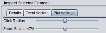
You can zoom in and out by using either the mouse wheel or the Zoom Factor slider. When clicking on a displayed item SEAMCAT tries to match the coordinates of the click to a cellular element – selecting the first matched item.
When SEAMCAT tries to match the click to an element it allows for a certain amount of uncertainty when matching the coordinates. This uncertainty is also called click radius to illustrate the effect of the actual click point being in the centre of a circle used to search for CDMA elements. You can adjust the “click radius” and in combination with the zoom this allows for all elements to be selected using the algorithm supplied above.
It is often the case that an element different than desired or no element at all is selected when clicking the plot. This problem is resolved by zooming in and possibly changing the click radius.
12.9 Interference calculations
12.9.1 Introduction
The Interference Calculation Engine (ICE) is that part of the SEAMCAT architecture which calculates for generic victim receiver the probability of being impacted by the sum of the simulated interference power. The calculated result is commonly called "Interference probability" or " probability of interference", in fact it is the probability of exceeding the limit of one of the interference criteria given for the victim receiver.
Regarding the definition of the Radio Regulations (RR) Article 1.166
The effect of unwanted energy due to one or a combination of emissions, radiations, or inductions upon reception in a radiocommunication system, manifested by any performance degradation, misinterpretation, or loss of information which could be extracted in the absence of such unwanted energy.
Administrations may have to distinguish between permissible interference (RR 1.167) and accepted interference (RR 1.168).
Details of the interference calculation algorithm are given in ANNEX 2:.
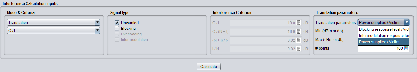
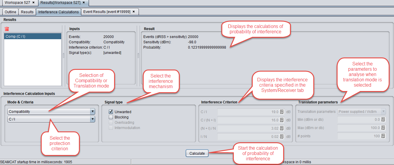
12.9.2 Interference calculation GUI
When the simulation is finished, the dRSS and the iRSS vectors are stored. You may proceed to use the facilities of the Interference Calculation Engine (ICE) in order to evaluate the probability of interference for the simulated scenario.
The probability of interference is calculated by the ICE with the following choice of input parameters:
-
Calculation mode: compatibility or translation;
-
Which type of interference signal is considered for calculation: unwanted, blocking, intermodulation, overloading or their combination;
-
Interference criterion: C/I, C/(N+I), (N+I)/N or I/N.
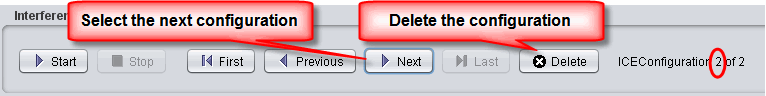
If more than one interference calculation was done (i.e. with different combination of interference criterion), you may scroll through all of them by using the Previous / Next buttons.
Interference calculation results:
-
single interference probability value (compatiblity mode);
-
probability as function of the translation parameter (translation mode).
When the compatiblity mode is chosen, a single-figure estimate of the probability of interference is calculated;
When the Translation mode is chosen, you may calculate and display as chart the probability of interference as function of one of the following input parameters:
-
Output power of Interfering transmitter;
-
Blocking response level of Victim receiver;
-
Intermodulation response level of Victim receiver.
You are able to save the results of the translation mode using the “save translation button”.

|
ID |
Description |
Comments |
|
1 |
Calculation mode/ |
Compatibility: Gives the probability of being interfered by the Blocking interference and/or by the Unwanted interference and/or by intermodulation interference. |
|
2 |
Calculation mode/ |
In this case all the following parameters should be independent from frequencies: Receiver blocking response mask, Receiver intermodulation rejection mask, power distribution of interfering transmitter, Unwanted emission floor mask. Calculation of the probability of interference as a function of the reference parameters (Power supplied by the It for the unwanted, Blocking response level of the Vr for the Blocking, And intermodulation rejection level for the Vr). These parameters are varying on user-defined definition domain defined by the number of points where the software has to calculate the probability. |
|
3 |
Signal type |
Choose the interference studied: Unwanted and/or Blocking and/or Intermodulation and Overloading in case simulated. |
|
4 |
Interference criterion |
Choose between C/I, C/(N+I), (N+I)/N, I/N) |
|
5 |
Events |
Total number of simulated events, |
|
6 |
Events (dRSS > sensitivity) |
It represents the number of events taken into account for the calculation. The accuracy of the calculated results relates to this ratio, i.e. the less this number the higher the inaccuracy. |
|
7 |
Calculation control |
Delete a result, and see the last results |
|
8 |
Translation parameters: If translation was chosen |
Number of points between the min and max, where the software will calculate the probability. |
|
9 |
Result / Compatibility |
Probability of interference: 1 - always interfered, 0 - never interfered |
|
10 |
Result / Translation |
Gives the graph, showing the resulting probability of interference vs. the selected values of translation parameter. The average of the graph depends of the number of points, but the higher the number is, the longer the calculations are. |
|
11 |
Save translation button |
You are able to save the results of the translation mode |

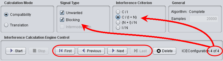
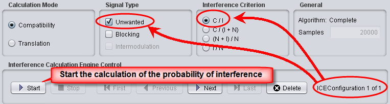
12.9.3 Interference Calculation Engine Control
It allows to the calculation of the probability of interference for several ICE configurations (i.e. different signal types, interference criteria, etc..) for the same simulation. Figure 272 presents how the control box is used.
|
|
|---|
|
|
|---|
|
(a) |
|
|
|
(b) |
|
|
|
(c) |
|
Figure 272: Use of the Interference Calculation Engine (ICE)
|
When the translation mode is activated, the overloading feature is deactivated as shown in Figure 273.