12.4 Spectrum sensing results
- Introduction
- 12.4.1 sRSS vector
- 12.4.2 WSD frequency
- 12.4.3 WSD e.i.r.p.
- 12.4.4 Victim frequency vector
- 12.4.5 Average e.i.r.p. per frequency
- 12.4.6 Average active WSDs per frequency vector
Introduction
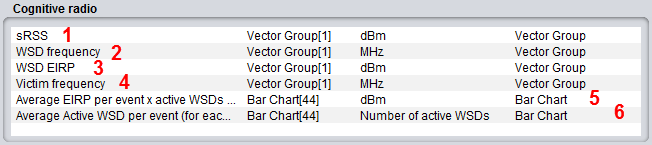
When the cognitive radio mode is activated, SEAMCAT resturns the output vector shown in Figure 251 and described in Table 52.
|
# |
Item |
Description |
|
1 |
sRSS |
sRSS value calculated at the selected WSD frequency (i.e. where the WSD is allowed to transmit) for each of the event |
|
2 |
WSD frequency |
The actual selected frequency at which the WSDs are allowed to transmit as the result of the spectrum sensing algorithm |
|
3 |
WSD e.i.r.p. |
The actual selected e.i.r.p. at which the WSDs are allowed to transmit as the result of the spectrum sensing algorithm |
|
4 |
Victim frequency |
frequency at which the victim device transmits per event |
|
5 |
Average e.i.r.p. per event x active WSDs (for each frequency) |
average e.i.r.p. per event for all the active WSDs transmitting at a certain frequency |
|
6 |
Average Active WSD per event (for each frequency) |
|
At the end of the simulation, SEAMCAT provides a set of output vectors as above. Then you can perform the interference probability calculation as previously described.
12.4.1 sRSS vector
The sRSS vector (dBm) is merely the sRSS value calculated at the selected WSD frequency (i.e. where the WSD is allowed to transmit) for each of the event. Figure 252 displays the vector for each WSD. You can select any or all of the WSD (#1). The same applies to the CDF and density graphs (#2).
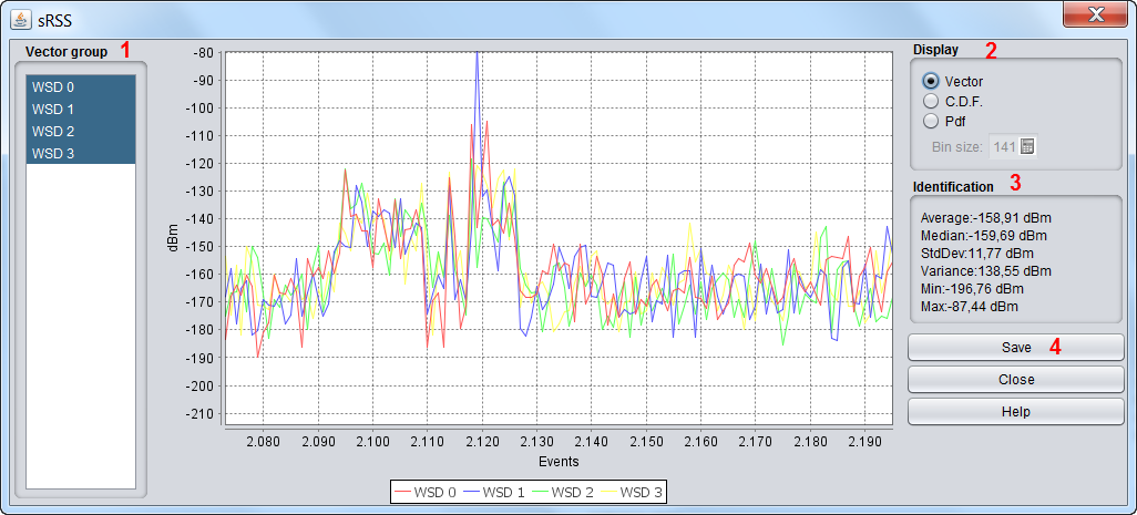
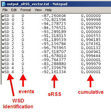
You are able to save the results (#4) as .txt file for further post-processing.
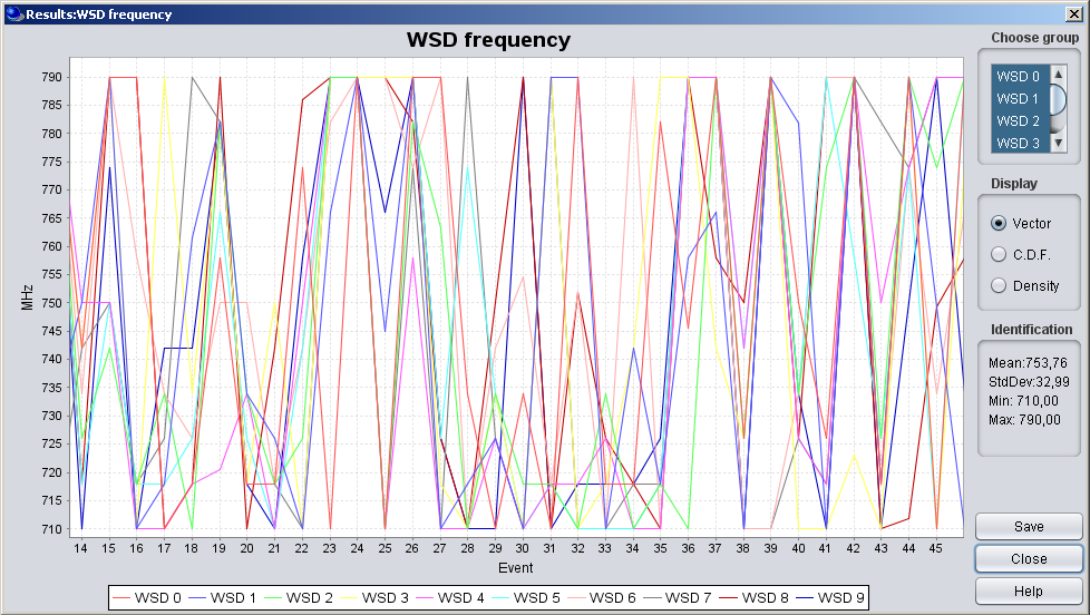
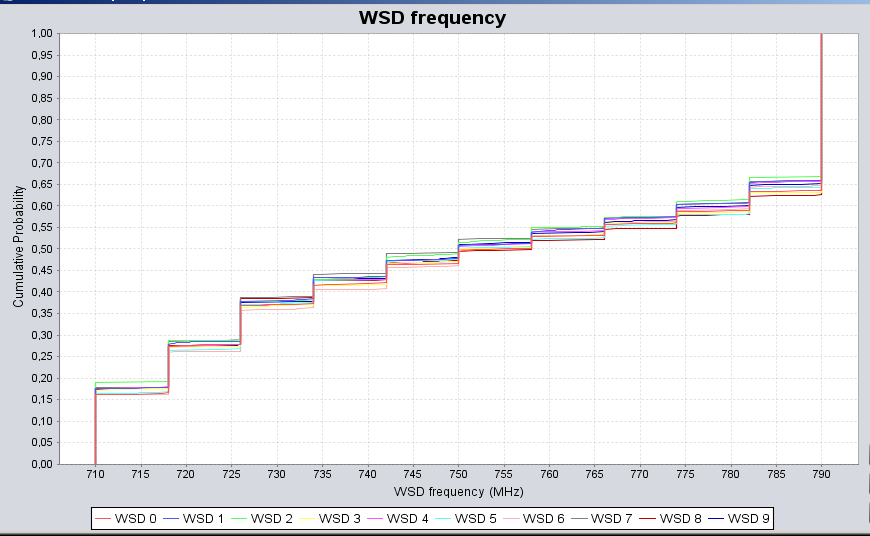
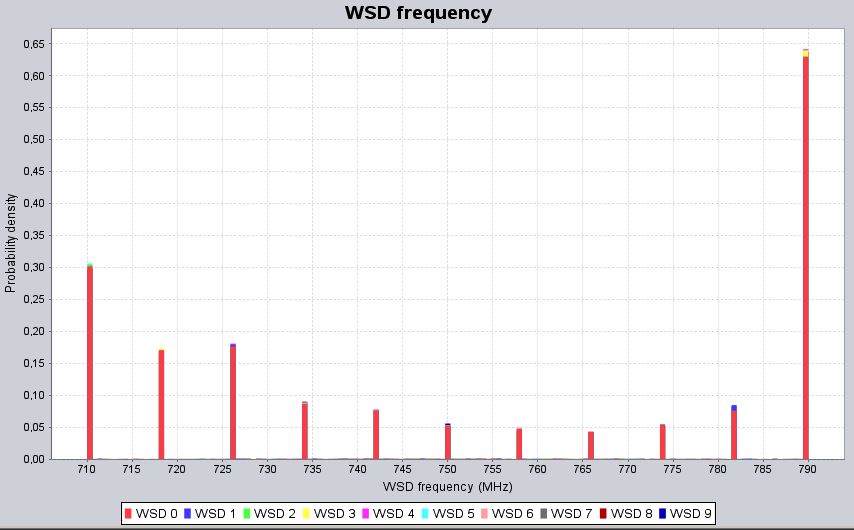
12.4.2 WSD frequency
This vector represents the actual selected frequency (MHz) at which the WSDs are allowed to transmit as the result of the spectrum sensing algorithm.
|
|
|
|---|---|
|
(a) |
(b) |
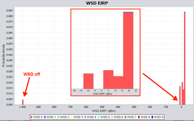
12.4.3 WSD e.i.r.p.
The actual selected e.i.r.p. (dBm) at which the WSDs are allowed to transmit as the result of the spectrum sensing algorithm. This vector displays the e.i.r.p. for each of the WSD for all the events. In the example presented in Figure 256, the WSDs are transmitting with a e.i.r.p. between -10 and 20 dBm and -1000 dBm (equivalent to WSD switch off).
12.4.4 Victim frequency vector
The victim frequency vector (MHz) represents the frequency at which the victim device transmits per event.
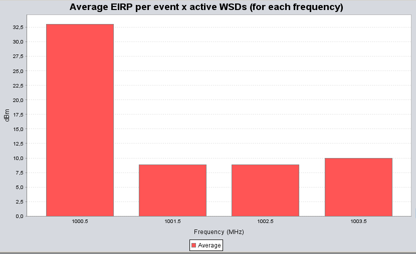
12.4.5 Average e.i.r.p. per frequency
It presents the average e.i.r.p. per event (dBm vs MHz) for all the active WSDs transmitting at a certain frequency such that:
 (Eq. 68)
Let us assume a different example from above, where 4 channels have been identified for the WSD to operate. Figure 257 shows that on average 33 dBm, for one event, was transmitted by the active WSDs at 1000.5 MHz , 8.82 dBm at 1001.5 MHz etc...
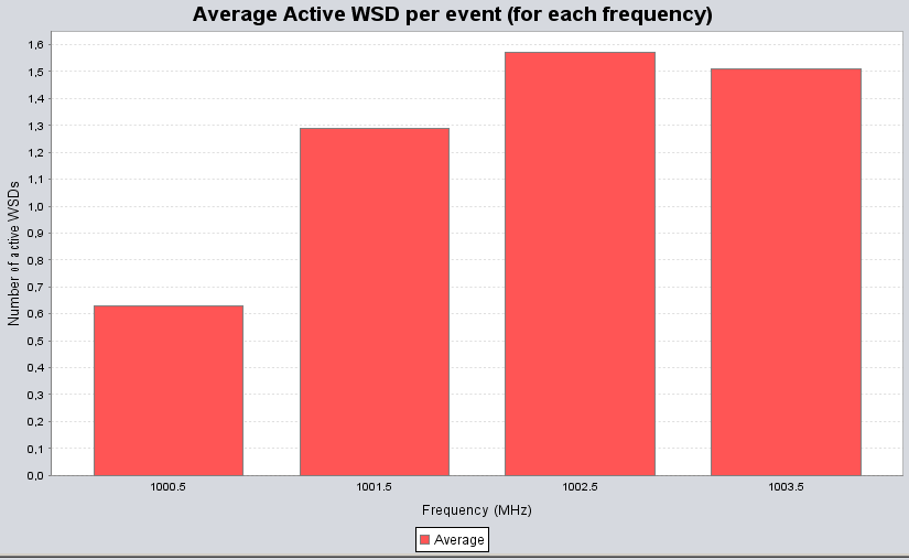
12.4.6 Average active WSDs per frequency vector
It provides the average number of active WSD per event for a specific frequency:
 (Eq. 69)
Re-using the example of Figure 257, Figure 258 indicates that, with for instance 5 WSDs set as input parameters, an average of 0.63 WSDs were active at 1000.5 MHz (with 33 dBm e.i.r.p. Figure 257), 1.29 WSDs were active at 1001.5 MHz (with 8.82 dBm e.i.r.p. Figure 257), 1.57 active WSDs at 1002.5 MHz and 1.51 active WSDs at 1003.5 MHz. It can also be noted that in this particular example, the sum of the active WSDs across the selected frequencies is 5, meaning that all the simulated WSDs have been active and none have been turn off.