| **Description** | **Symbol** | **Type** | **Unit** | **Comments** |
| Frequency | fVLT or fILT | Distribution or Scalar | MHz | Distribution of the centre frequency of the victim system or the interfering system links. |
[](https://wiki.cept.org/uploads/images/gallery/2026-04/EhlWsRWoCrP9me2p-image.png)
 | Add an interfering systems link to the scenario | [](https://wiki.cept.org/uploads/images/gallery/2026-04/iX5WAtkuje0mcG8y-image.png)
 | Generate multiple interfering links |
[](https://wiki.cept.org/uploads/images/gallery/2026-04/Ze3FwAAQwVCKm7ke-image.png)
 | Duplicate an interfering link |  | Change the selected system type |
 | Delete a link | [](https://wiki.cept.org/uploads/images/gallery/2026-04/lF5iK2TjSTNr4mfn-image.png)
 | On-line manual help |
| **Description** | **Symbol** | **Type** | **Unit** | **Comments** |
| Circular or hexagonal layout | - | - | - | General circular or hexagonal layout |
| Number of tiers of generated multiple cells | - | Scalar | - | You can generate as many tiers as you want |
| Number of links in the first tier | - | Scalar | - | You can set the total number of links in the first tier |
| Intersite distance | D | Scalar | Km | Distance between 2 BSs |
| Displacement angle | θ | Scalar | Degree | Angle between the horizontal and the first BS (counter clockwise) |
| Angle offset | Scalar | Degree | Angle offset of the displacement angle |
| **Description** | **Symbol** | **Type** | **Unit** | **Comments** |
| **Reference component** | - | - | Positioning of the distributed component which is either the ILT or the ILR | |
| **Position relative to** | - | - | Positioning of the reference component relative to either the VLR or the VLT | |
| **Delta X** | ∆X | Distribution or Scalar | km | Horizontal distance between the transmitter and receiver. It can be used to shift horizontally the distributed receivers |
| **Delta Y** | ∆Y | Distribution or Scalar | km | Vertical distance between the transmitter and receiver. It can be used to shift vertically the distributed receivers |
| **Set ILR at he center of the ILT distribution** | - | Boolean | - | set the distance factor distribution of the ILT with regards to the VLR. It overwrites the settings in the transmitter to reveicer path of the interferer |
| **Path azimuth** | Distribution or Scalar | Deg | Horizontal angle for the location of the ILT respect to the victim link. If constant, the Rx’s location will be on a straight line. If not, the location of the Rx will be on an angular area. (See Annex A12.3) | |
| **Path distance factor** | Distribution or Scalar | Distance factor to describe path length between the ILT and VLR. This factor will be multiplied by Rsimu to obtain the coverage area. Therefore, the trialled distance between ILT and VLR will be Rsimu \*Path factor. E.g. if user enters a distribution 0…1, then the distance will be between 0 and Rsimu. If the path factor is constant, the ILT will be located on a circle around the VLR which means that the distance between the ILT and VLR will not change | ||
| **Simulation radius** | Rsimu | km | User defined | |
| **Number of active transmitter** | nactive | Scalar | If nactive>1, this will result in spatially-independent generation of the specified number of Its, whereas the resulting total iRSS strength will be obtained by simple power summation of the individual iRSS signal values. | |
| **Minimum coupling loss** | MCL | Distribution or Scalar | dB | The minimum path loss. It is used in the calculation of the effective path loss (Section 7.6) |
| **Protection distance** | d0 | Distribution or Scalar | (km) | minimum protection distance between the victim link receiver and interefering link transmitter (Section A13.2.3) |
| **Use of polygon** | You are also able to select a polygon shape as an alternative to the default circle. A various selection of polygon is available. You are able to rotate counter-clock wise (ccw) the polygon shape. | |||
| **Co-locate** | This feature allows deploying two interferers at the same location and their two transmitters could be transmitting at the same time while having different transmitter characteristics (e.g. emission mask, antenna radiation pattern…) |
| **Description** | **Symbol** | **Type** | **Unit** | **Comments** |
| Reference component | - | - | Positioning of the distributed component which is either the ILT or the ILR | |
| Position relative to | - | Boolean | - | Positioning of the Reference component relative to either the VLR or the VLT |
| Delta X | ∆X | Distribution or Scalar | km | Horizontal distance between the transmitter and receiver. It can be used to shift horizontally the distributed receivers. |
| Delta Y | ∆Y | Distribution or Scalar | km | Vertical distance between the transmitter and receiver. It can be used to shift vertically the distributed receivers. |
| set ILR at he center of the ILT distribution | - | Boolean | - | Set the distance factor distribution of the ILT with regards to the VLR. It overwrites the settings in the transmitter to reveicer path of the interferer. |
| Path azimuth | Distribution or Scalar | Deg | Horizontal angle for the location of the ILT respect to the victim link. If constant, the Rx’s location will be on a straight line. If not, the location of the Rx will be on an angular area. (See Annex A12.3) | |
| Number of active transmitter | nactive | Scalar | Number of active interferers in the simulation (nactive should be sufficiently large so that the (n+1)th interferer would bring a negligible additional interfering power). If nactive>1, this will result in spatially-independent generation of the specified number of Its, whereas the resulting total iRSS strength will be obtained by simple power summation of the individual iRSS signal values. | |
| Simulation radius | Rsimu | km | ***Note:** the simulation radius value is readable only after each simulation* | |
| Interferes density | A simulation radius is calculated, Rsimu. Interefering link transmitters will be randomly deployed within the area centred on the Victim link receiver and delimited by the simulation radius Rsimu. If a protection is defined then Interefering link transmitters will be randomly deployed within the area centred in the Victim link receiver and delimited by the protection distance and the simulation radius Rsimu . See Table 46 for information on the input parameter and Annex A13.2.2 for the calculation. | |||
| Minimum coupling loss | MCL | Distribution or Scalar | dB | The minimum path loss. It is used in the calculation of the effective path loss (Section 7.6) |
| Protection distance | d0 | Scalar | (km) | Minimum protection distance between the victim link receiver and interefering link transmitter (Section A13.2.3) |
| Co-locate | This feature allows deploying two interferers at the same location and their two transmitters could be transmitting at the same time while having different transmitter characteristics (e.g. emission mask, antenna radiation pattern…) |
| **Description** | **Symbol** | **Type** | **Unit** | **Comments** |
| Reference component | - | - | Positioning of the distributed component which is either the ILT or the ILR | |
| Position relative to | - | - | - | Positioning of the Reference component relative to either the VLR or the VLT |
| Delta X | ∆X | Distribution or Scalar | km | Horizontal distance between the transmitter and receiver. It can be used to shift horizontally the distributed receivers |
| Delta Y | ∆Y | Distribution or Scalar | km | Vertical distance between the transmitter and receiver. It can be used to shift vertically the distributed receivers |
| Set ILR at he center of the ILT distribution | - | Boolean | - | Set the distance factor distribution of the ILT with regards to the VLR. It overwrites the settings in the transmitter to reveicer path of the interferer |
| Path azimuth | Distribution or Scalar | Deg | Horizontal angle for the location of the ILT respect to the victim link. If constant, the Rx’s location will be on a straight line. If not, the location of the Rx will be on an angular area. (See Annex A1.1) | |
| Number of active transmitter | nactive | Scalar | Number of active interferers in the simulation (nactive should be sufficiently large so that the (n+1)th interferer would bring a negligible additional interfering power). If nactive>1, this will result in spatially-independent generation of the specified number of Its, whereas the resulting total iRSS strength will be obtained by simple power summation of the individual iRSS signal values | |
| Simulation radius | Rsimu | km | *Note: the simulation radius value is readable only after each simulation* | |
| Interferes density | The distance between the Victim link receiver and the Interefering link transmitter follows a Rayleigh distribution, where the standard deviation is given by . See Table 47 for information on the input parameter and Annex A13.2.4 for the calculation | |||
| Minimum coupling loss | MCL | Distribution or Scalar | dB | The minimum path loss. It is used in the calculation of the effective path loss (Section 7.6) |
| Protection distance | d0 | Scalar | (km) | minimum protection distance between the victim link receiver and interefering link transmitter (Section A13.2.3) |
| Co-locate | This feature allows deploying two interferers at the same location and their two transmitters could be transmitting at the same time while having different transmitter characteristics (e.g. emission mask, antenna radiation pattern…) |
| **Description** | **Symbol** | **Type** | **Unit** | **Comments** |
| Reference component | - | - | Positioning of the distributed component which is either the ILT or the ILR | |
| Position relative to | - | B | - | Positioning of the fixed interefer transmitter (ILT) or receiver (ILR) with the origin being. Reference component relative to either onthe VLR or the victim link transmitter (VLT) or receiver (VLR) on the option selected. |
| Delta X | ∆X | Distribution or Scalar | km | Horizontal distance between the transmitter and receiver. It can be used to shift horizontally the distributed receivers. |
| Delta Y | ∆Y | Distribution or Scalar | km | Vertical distance between the transmitter and receiver. It can be used to shift vertically the distributed receivers. |
| Minimum coupling loss | MCL | Distribution or Scalar | dB | The minimum path loss. It is used in the calculation of the effective path loss (Section 7.6) |
| **Description** | **Symbol** | **Type** | **Unit** | **Comments** |
| Position relative to VLT or VLR | - | Boolean | - | Positioning of the fixed interefer transmitter (ILT) or receiver (ILR) with the origin being either on the victim link transmitter (VLT) or receiver (VLR) on the option selected. |
| Delta X | ∆X | Distribution or Scalar | km | Horizontal distance between the transmitter and receiver. It can be used to shift horizontally the distributed receivers. |
| Delta Y | ∆Y | Distribution or Scalar | km | Vertical distance between the transmitter and receiver. It can be used to shift vertically the distributed receivers. |
| Path azimuth | - | Distribution or Scalar | Deg | Horizontal angle for the location of the interfering BS ref.cell respect to the VLR or VLT |
| Path distance | - | Distribution or Scalar | km | Path length between the interfering BS ref.cell respect to the VLR or VLT |
| Minimum coupling loss | MCL | Distribution or Scalar | dB | The minimum path loss. It is used in the calculation of the effective path loss (Section 7.6) |
| **Description** | **Symbol** | **Type** | **Unit** | **Comments** |
| **Density of transmitters** | densit | Scalar | 1/km2 | Maximum number of active transmitters per km2 |
| **Probability of transmission** | Pit | Scalar | % | |
| **Activity** | activityit | Function (X,Y) | 1/h | Temporal activity variation as a function of the time of the day (hh/mm/ss) |
| **Time** | time | Scalar | hour | Time of the day. If the activity function (above), here it should be specified which hour (from the defined range of function) should be considered in a simulation |
| **Description** | **Symbol** | **Type** | **Unit** | **Comments** |
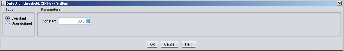
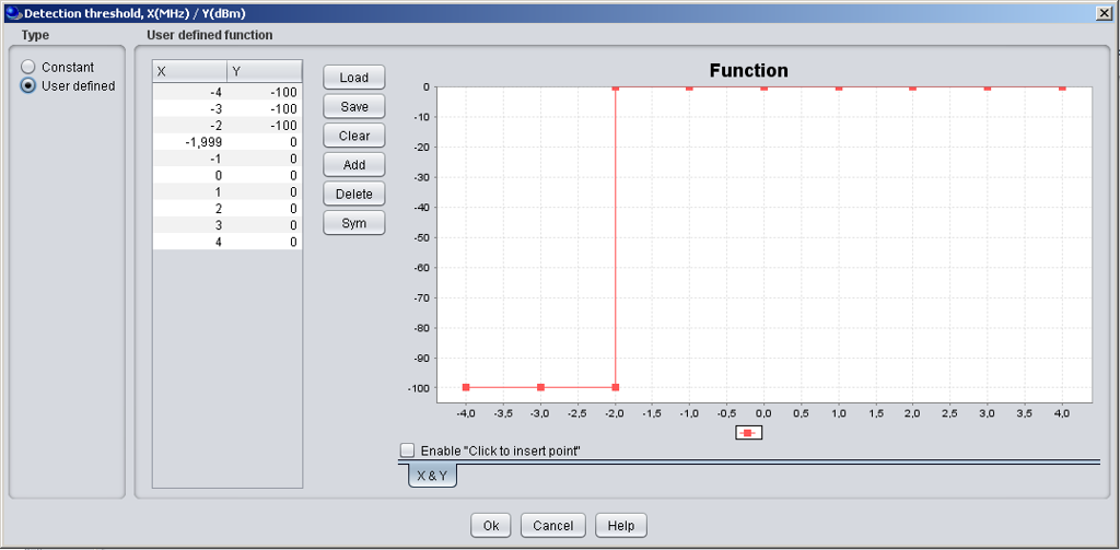
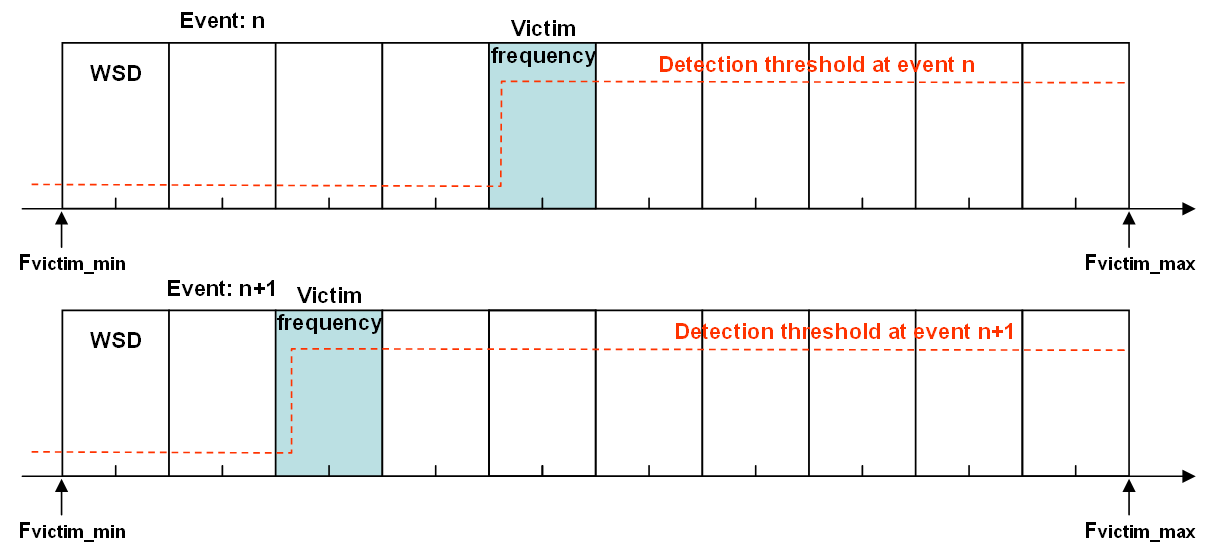
| **Detection threshold:** | Function (X,Y) or Scalar (offset) | dBm | Define the detection threshold for the spectrum sensing in a offset function. Either a constant value (i.e. flat over the spectrum) or as a user defined function as shown in #1 of Figure 232 illustrates the setting of the detection threshold (a) as a constant or (b) as a function. Figure 233 (c) illustrates where the offset refers to. Note the user-defined function is defined as offset with the victim frequency being the reference. The offset 0 is refered to the Victim frequency. | |
| **Probability of failure:** | Scalar | % | You can select this function as shown in **\#2** of Figure 232. The probability of failure is given in percentage. In the illustration below a probability of failure of 10% is entered. Positive value from 0 to 100. | |
| **Sensing reception bandwidth** | Scalar | kHz | Define the bandwidth of the sensing device (i.e. ILT). It is used in the calculation of the sRSS: This is a constant value given in kHz as shown in **\#3** of Figure 232. | |
| **e.i.r.p. max In-block limit** | Function (X,Y) (offset) | Offset (MHz)/ Mask (dBm)/ Ref.BW (kHz) | Define the E.I.R.Pmax In-block limit to protect the victim system as an offset function where the offset 0 is refered to the selected interfering frequency. The outcome of the algorithm set the allowed power at the ILT. It has the following components \[offset, Mask, Ref.BW\] where Offset in MHz is equivalent to the “DTT in use at” columns, Mask in dBm is the “In-block CR EIRPmax limit” and Ref. BW is the bandwidth of the DTT as shown in **\#4** of Figure 232. Note that SEAMCAT will normalise any value entered in the table to 1 MHz and convert back to the victim bandwidth. |
| [](https://wiki.cept.org/uploads/images/gallery/2026-04/igmO47RiVILV7jVk-image.png) |
|---|
| **(a)** |
| [](https://wiki.cept.org/uploads/images/gallery/2026-04/uy1wfZFg5BM3WWnY-image.png)
 |
| **(b)** |
| [](https://wiki.cept.org/uploads/images/gallery/2026-04/gbA7Cf1gDX4x2NxX-image.png)
 |
| **(c)** |
| **Figure 233: Example of the detection threshold (a) as a constant or (b) as a function and illustrates in (c) where the offset refers to** |
| **DTT in use at** | **In-block CR e.i.r.p. max limit (dBm)** |
| co-channel | -¥¥ |
| *n* ± 1 | -12.8 |
| *n* ± 2 | 3.2 |
| *n* ± 3 | 11.2 |
| *n* ± 4 | 16.2 |
| *n* ± 5 | 20.2 |
| *n* - 6 | 16.2 |
| *n* + 6 | 21.2 |
| *n* ± 7 | 22.2 |
| *n* ± 8 | 23.2 |
| *n* - 9 | 4.2 |
| *n* + 9 | 23.2 |
| *n* ± 10 | 24.2 |
| *> n* ± 11 | 25.2 |