10.3 Interfering Link Transmitter to Victim Link Receiver Path (ILT -> VLR)

introduction
10.3.1 Relative positioning of interfering link (Generic system)
10.3.2 Relative positioning of interfering link (Cellular system)
10.3.3 Interferers density
10.3.4 Pathloss correlation
10.3.5 Propagation Model

introduction

The ILT to VLR path can have several combinations as shown in Figure 224. Four panels characterised the path between the ILT and ILR.

Figure 221: ILT to VLR path combination with generic and cellular system

Figure 222: Transmitter to Victim Link Receiver Path (ILT -> VLR)

10.3.1 Relative positioning of interfering link (Generic system)

The relative position of the Victim Receiver (VLR) and the Interfering Transmitter (ILT) depends on the various options presented below. There is a unique simulation radius (R_simu) contrary to the 2 coverage radius (one for the victim and one for the interferer link). This is illustrated below in Figure 223 for a generic system interfering with a second generic system.

See ‎ANNEX 12: for further details on the algorithm and conventions.

Figure 223: Example of the simulation radius (VLR with ILT)

Depending on the system simulated several positioning options are possible when the generic system is the interferer and the victim is a generic system and cellular system as shown in Figure 224 and Figure 227 respectively.

Figure 224: Relative positioning of a generic interfering link with a generic victim system

Each interfering signal calculation results from the contribution of

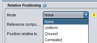
None: n_active interefering link transmitters located in a circular area with the simulation radius. You define yourself the radius. The random placement of the interefering link transmitters in this area is defined by the path azimuth and the path distance factor parameters.

See Annex ‎A13.2.1 for detailed algorithm.

Table 42: ILT-VLR path - none mode (generic vs generic)

Description	Symbol	Type	Unit	Comments
Reference component	-		-	Positioning of the distributed component which is either the ILT or the ILR
Position relative to	-		-	Positioning of the reference component relative to either the VLR or the VLT
Delta X	∆X	Distribution or Scalar	km	Horizontal distance between the transmitter and receiver. It can be used to shift horizontally the distributed receivers
Delta Y	∆Y	Distribution or Scalar	km	Vertical distance between the transmitter and receiver. It can be used to shift vertically the distributed receivers
Set ILR at he center of the ILT distribution	-	Boolean	-	set the distance factor distribution of the ILT with regards to the VLR. It overwrites the settings in the transmitter to reveicer path of the interferer
Path azimuth		Distribution or Scalar	Deg	Horizontal angle for the location of the ILT respect to the victim link. If constant, the Rx’s location will be on a straight line. If not, the location of the Rx will be on an angular area. (See Annex ‎A12.3)
Path distance factor		Distribution or Scalar		Distance factor to describe path length between the ILT and VLR. This factor will be multiplied by R_simu to obtain the coverage area. Therefore, the trialled distance between ILT and VLR will be R_simu *Path factor. E.g. if user enters a distribution 0…1, then the distance will be between 0 and R_simu. If the path factor is constant, the ILT will be located on a circle around the VLR which means that the distance between the ILT and VLR will not change
Simulation radius	R_simu		km	User defined
Number of active transmitter	n_active	Scalar		If n_active>1, this will result in spatially-independent generation of the specified number of Its, whereas the resulting total iRSS strength will be obtained by simple power summation of the individual iRSS signal values.
Minimum coupling loss	MCL	Distribution or Scalar	dB	The minimum path loss. It is used in the calculation of the effective path loss (Section ‎7.6)
Protection distance	d0	Distribution or Scalar	(km)	minimum protection distance between the victim link receiver and interefering link transmitter (Section ‎A13.2.3)
Use of polygon				You are also able to select a polygon shape as an alternative to the default circle. A various selection of polygon is available. You are able to rotate counter-clock wise (ccw) the polygon shape.
Co-locate				This feature allows deploying two interferers at the same location and their two transmitters could be transmitting at the same time while having different transmitter characteristics (e.g. emission mask, antenna radiation pattern…)

Uniform density: Each interfering signal calculation results from the contribution of n_active interefering link transmitters uniformly located in a circular area. The parameters are taken from the system settings (see section A13.2.2.)

Figure 225: Transmitter density and traffic

Table 43: ILT-VLR path - Uniform density mode (generic vs generic)

Description	Symbol	Type	Unit	Comments
Reference component	-		-	Positioning of the distributed component which is either the ILT or the ILR
Position relative to	-	Boolean	-	Positioning of the Reference component relative to either the VLR or the VLT
Delta X	∆X	Distribution or Scalar	km	Horizontal distance between the transmitter and receiver. It can be used to shift horizontally the distributed receivers.
Delta Y	∆Y	Distribution or Scalar	km	Vertical distance between the transmitter and receiver. It can be used to shift vertically the distributed receivers.
set ILR at he center of the ILT distribution	-	Boolean	-	Set the distance factor distribution of the ILT with regards to the VLR. It overwrites the settings in the transmitter to reveicer path of the interferer.
Path azimuth		Distribution or Scalar	Deg	Horizontal angle for the location of the ILT respect to the victim link. If constant, the Rx’s location will be on a straight line. If not, the location of the Rx will be on an angular area. (See Annex ‎A12.3)
Number of active transmitter	nactive	Scalar		Number of active interferers in the simulation (nactive should be sufficiently large so that the (n+1)th interferer would bring a negligible additional interfering power). If n_active>1, this will result in spatially-independent generation of the specified number of Its, whereas the resulting total iRSS strength will be obtained by simple power summation of the individual iRSS signal values.
Simulation radius	R_simu		km	Note: the simulation radius value is readable only after each simulation
Interferes density				A simulation radius is calculated, R_simu. Interefering link transmitters will be randomly deployed within the area centred on the Victim link receiver and delimited by the simulation radius R_simu. If a protection is defined then Interefering link transmitters will be randomly deployed within the area centred in the Victim link receiver and delimited by the protection distance and the simulation radius R_simu . See Table 46 for information on the input parameter and Annex ‎A13.2.2 for the calculation.
Minimum coupling loss	MCL	Distribution or Scalar	dB	The minimum path loss. It is used in the calculation of the effective path loss (Section ‎7.6)
Protection distance	d0	Scalar	(km)	Minimum protection distance between the victim link receiver and interefering link transmitter (Section ‎A13.2.3)
Co-locate				This feature allows deploying two interferers at the same location and their two transmitters could be transmitting at the same time while having different transmitter characteristics (e.g. emission mask, antenna radiation pattern…)

Closest interferer: Each interfering signal calculation results from the contribution of just one interefering link transmitter. This ILT is randomly placed in a circular area with a simulation radius derived from the density of interferers. See Annex ‎A13.2.4 for detailed alogorithm. The parameters are taken from the system settings (see section A13.2.4).

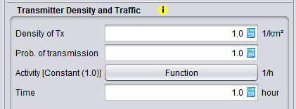
Figure 226: Transmitter density and traffic

Table 44: ILT-VLR path - Closest interferer mode (generic vs generic)

Description	Symbol	Type	Unit	Comments
Reference component	-		-	Positioning of the distributed component which is either the ILT or the ILR
Position relative to	-	-	-	Positioning of the Reference component relative to either the VLR or the VLT
Delta X	∆X	Distribution or Scalar	km	Horizontal distance between the transmitter and receiver. It can be used to shift horizontally the distributed receivers
Delta Y	∆Y	Distribution or Scalar	km	Vertical distance between the transmitter and receiver. It can be used to shift vertically the distributed receivers
Set ILR at he center of the ILT distribution	-	Boolean	-	Set the distance factor distribution of the ILT with regards to the VLR. It overwrites the settings in the transmitter to reveicer path of the interferer
Path azimuth		Distribution or Scalar	Deg	Horizontal angle for the location of the ILT respect to the victim link. If constant, the Rx’s location will be on a straight line. If not, the location of the Rx will be on an angular area. (See Annex ‎A1.1)
Number of active transmitter	nactive	Scalar		Number of active interferers in the simulation (nactive should be sufficiently large so that the (n+1)th interferer would bring a negligible additional interfering power). If n_active>1, this will result in spatially-independent generation of the specified number of Its, whereas the resulting total iRSS strength will be obtained by simple power summation of the individual iRSS signal values
Simulation radius	R_simu		km	Note: the simulation radius value is readable only after each simulation
Interferes density				The distance between the Victim link receiver and the Interefering link transmitter follows a Rayleigh distribution, where the standard deviation is given by . See Table 47 for information on the input parameter and Annex ‎A13.2.4 for the calculation
Minimum coupling loss	MCL	Distribution or Scalar	dB	The minimum path loss. It is used in the calculation of the effective path loss (Section ‎7.6)
Protection distance	d0	Scalar	(km)	minimum protection distance between the victim link receiver and interefering link transmitter (Section ‎A13.2.3)
Co-locate				This feature allows deploying two interferers at the same location and their two transmitters could be transmitting at the same time while having different transmitter characteristics (e.g. emission mask, antenna radiation pattern…)

- Correlated : It is called the correlated mode. It means that the positions of the receiver and transmitter are geographically fixed with respect to each other (e.g. co-located or constantly spaced base stations). In the following four cases of fixed placement, the relative location of the two pair of transmitter and receiver is described by dX/dY displacement, with the origin being either on the Transmitter or Receiver of the victim link depending on the option selected;

Table 45: ILT-VLR path – Correlated mode (generic vs generic)

Description	Symbol	Type	Unit	Comments
Reference component	-		-	Positioning of the distributed component which is either the ILT or the ILR
Position relative to	-	B	-	Positioning of the fixed interefer transmitter (ILT) or receiver (ILR) with the origin being. Reference component relative to either onthe VLR or the victim link transmitter (VLT) or receiver (VLR) on the option selected.
Delta X	∆X	Distribution or Scalar	km	Horizontal distance between the transmitter and receiver. It can be used to shift horizontally the distributed receivers.
Delta Y	∆Y	Distribution or Scalar	km	Vertical distance between the transmitter and receiver. It can be used to shift vertically the distributed receivers.
Minimum coupling loss	MCL	Distribution or Scalar	dB	The minimum path loss. It is used in the calculation of the effective path loss (Section ‎7.6)

In the case the victim system is a cellular system (CDMA or OFDMA, either UL or DL), the options are slightly changed as shown below, where Position relative to is always the BS of the reference cell.

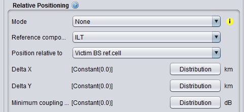
Figure 227: Relative positioning of a generic interfering link with a cellular victim system

10.3.2 Relative positioning of interfering link (Cellular system)

The relative position of the Victim Receiver (VLR) and the Interfering cellular system depends on the various options presented below.

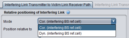
Figure 228: Relative positioning of a cellular interfering link with a generic victim system

Cor. (interfering BS ref. cell): in which case the relative location is explicitely defined by the dX/dY values given in the scenario and the reference is the BS ref.cell. It is a similar mode as described in Table 43 where the BS ref.cell of the cellular interferer is position with respect to the VLT or VLR depending on the selection;
Dyn (interfering BS ref.cell): this dynamic distance mode provides a a relative location that follows a uniform distribution in the distance and angle domain.

Table 46: ILT-VLR path – Correlated mode (cellular vs generic)

Description	Symbol	Type	Unit	Comments
Position relative to VLT or VLR	-	Boolean	-	Positioning of the fixed interefer transmitter (ILT) or receiver (ILR) with the origin being either on the victim link transmitter (VLT) or receiver (VLR) on the option selected.
Delta X	∆X	Distribution or Scalar	km	Horizontal distance between the transmitter and receiver. It can be used to shift horizontally the distributed receivers.
Delta Y	∆Y	Distribution or Scalar	km	Vertical distance between the transmitter and receiver. It can be used to shift vertically the distributed receivers.
Path azimuth	-	Distribution or Scalar	Deg	Horizontal angle for the location of the interfering BS ref.cell respect to the VLR or VLT
Path distance	-	Distribution or Scalar	km	Path length between the interfering BS ref.cell respect to the VLR or VLT
Minimum coupling loss	MCL	Distribution or Scalar	dB	The minimum path loss. It is used in the calculation of the effective path loss (Section ‎7.6)

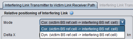
Figure 229: Relative positioning of a cellular interfering link with a cellular victim system

Cor. (victim BS ref.cell à interfering BS ref.cell): It is the same mode as described in Table 45 but where the BS of the reference cell of the victim cellular network is the reference position of the BS of the reference cell of the interfering cellular network.
Dyn. (victim BS ref.cell à interfering BS ref.cell): It is the same mode as described in Table 48, but where the BS of the reference cell of the victim cellular network is the reference position of the BS of the reference cell of the interfering cellular network.

10.3.3 Interferers density

The panel is activated if "Uniform density" or/and "closest interferer" mode is selected. See Annex ‎A13.2.2 for more details on the calculation.

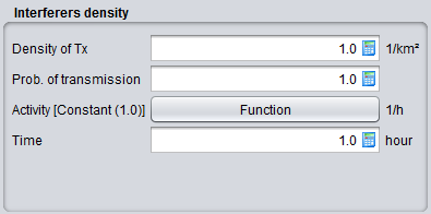Figure 230: Interferers density panel (only in "Uniform density" and "closest interferer” mode)

Table 47: Setting up the interferes density

Description	Symbol	Type	Unit	Comments
Density of transmitters	dens_it	Scalar	1/km²	Maximum number of active transmitters per km²
Probability of transmission	P_it	Scalar	%
Activity	activity_it	Function (X,Y)	1/h	Temporal activity variation as a function of the time of the day (hh/mm/ss)
Time	time	Scalar	hour	Time of the day. If the activity function (above), here it should be specified which hour (from the defined range of function) should be considered in a simulation

10.3.4 Pathloss correlation

The panel is activated if the victim is either OFDMA UL or OFDMA DL. It is decribed in more details in Section ‎9.11.

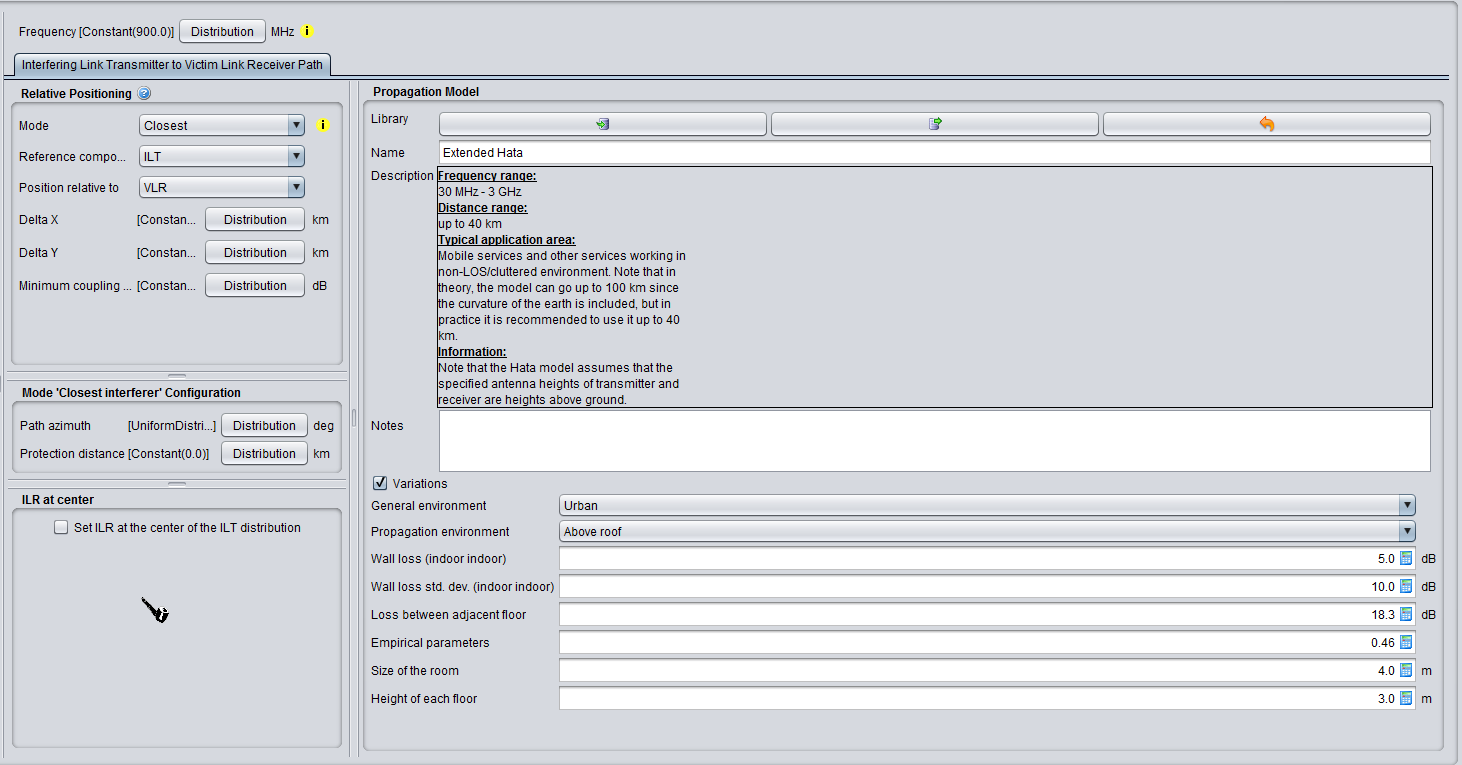
10.3.5 Propagation Model

You can choose the suitable propagation model to be applied when calculating signal loss between the ILT and the VLR. A choice and settings of propagation models are presented in ‎ANNEX 17:.